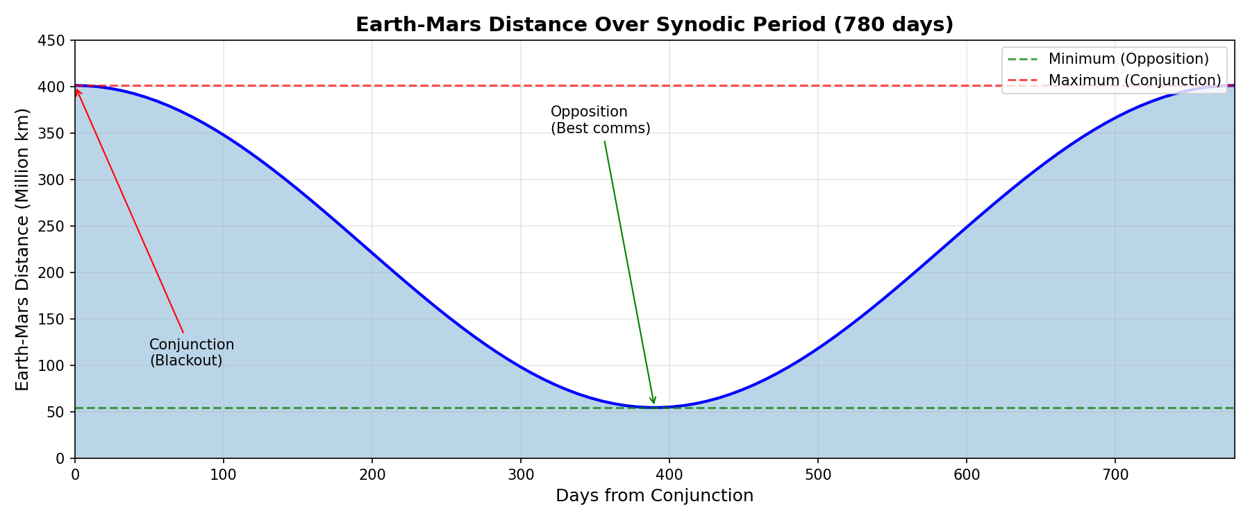
Mars orbits the Sun at a different speed than Earth, meaning the distance between them constantly changes over a 780-day cycle:
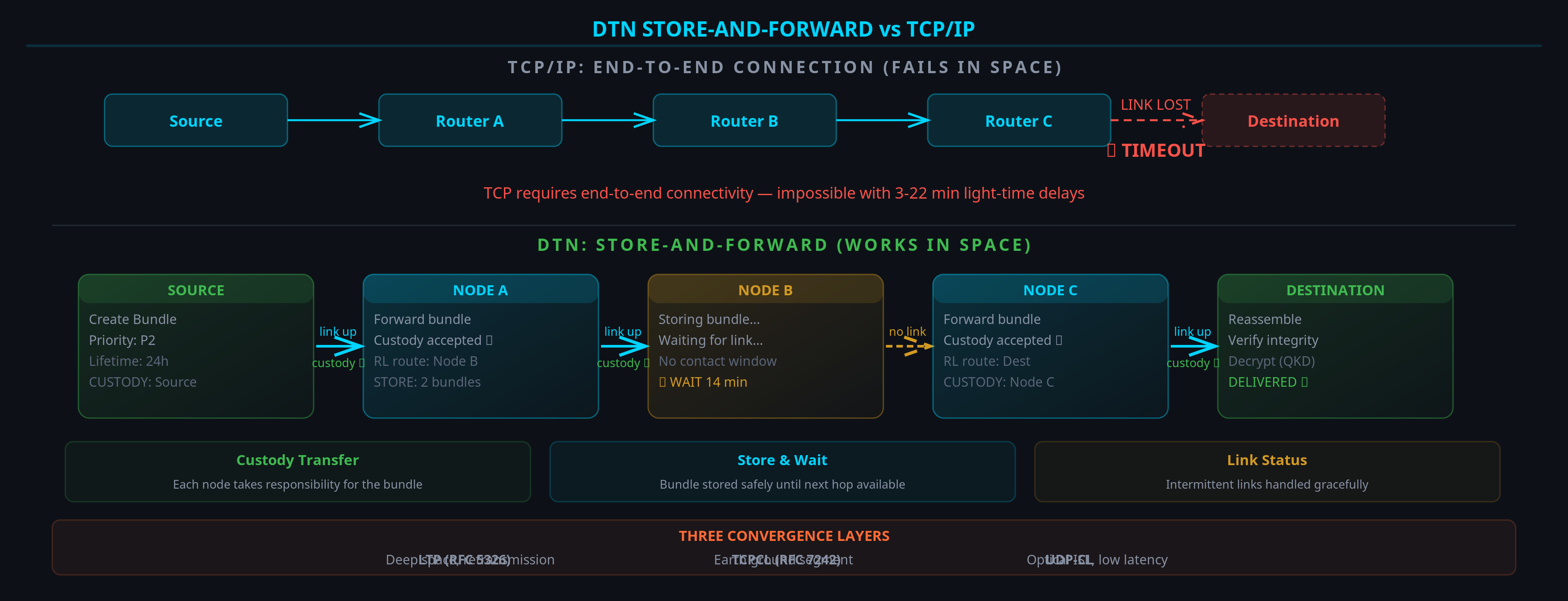
TCP/IP — the protocol that powers the internet — assumes instant responses and continuous connections. In space, those assumptions break down:
Delay-Tolerant Networking
Messages are packaged into “bundles” that hop from node to node, waiting at each stop until the next connection is available. Like postal mail — not a phone call.
AI-Powered Routing
Instead of fixed routing tables, our AI agent learns the best paths through the network by trial and error, adapting to changing conditions in real time.
Quantum Security
Using the laws of quantum physics to create unbreakable encryption. Any eavesdropping attempt is physically detectable — secured by nature itself.
Optical Communications
Using infrared lasers instead of radio waves for 10–100× faster data transfer. Like upgrading from dial-up to fiber optic — in space.
What is Delay-Tolerant Networking?
The technology that makes interplanetary communication possible — sending data reliably across millions of kilometers, hours of delay, and intermittent connections.
- ✗ Instant response (< 1 second round trip)
- ✗ Continuous, unbroken connection
- ✗ Data arrives in perfect order
- ✗ Both sides active simultaneously
- ✓ 6 to 44 minute round-trip delay
- ✓ Intermittent, scheduled connections
- ✓ Data may arrive out of order
- ✓ 2-week solar conjunction blackouts
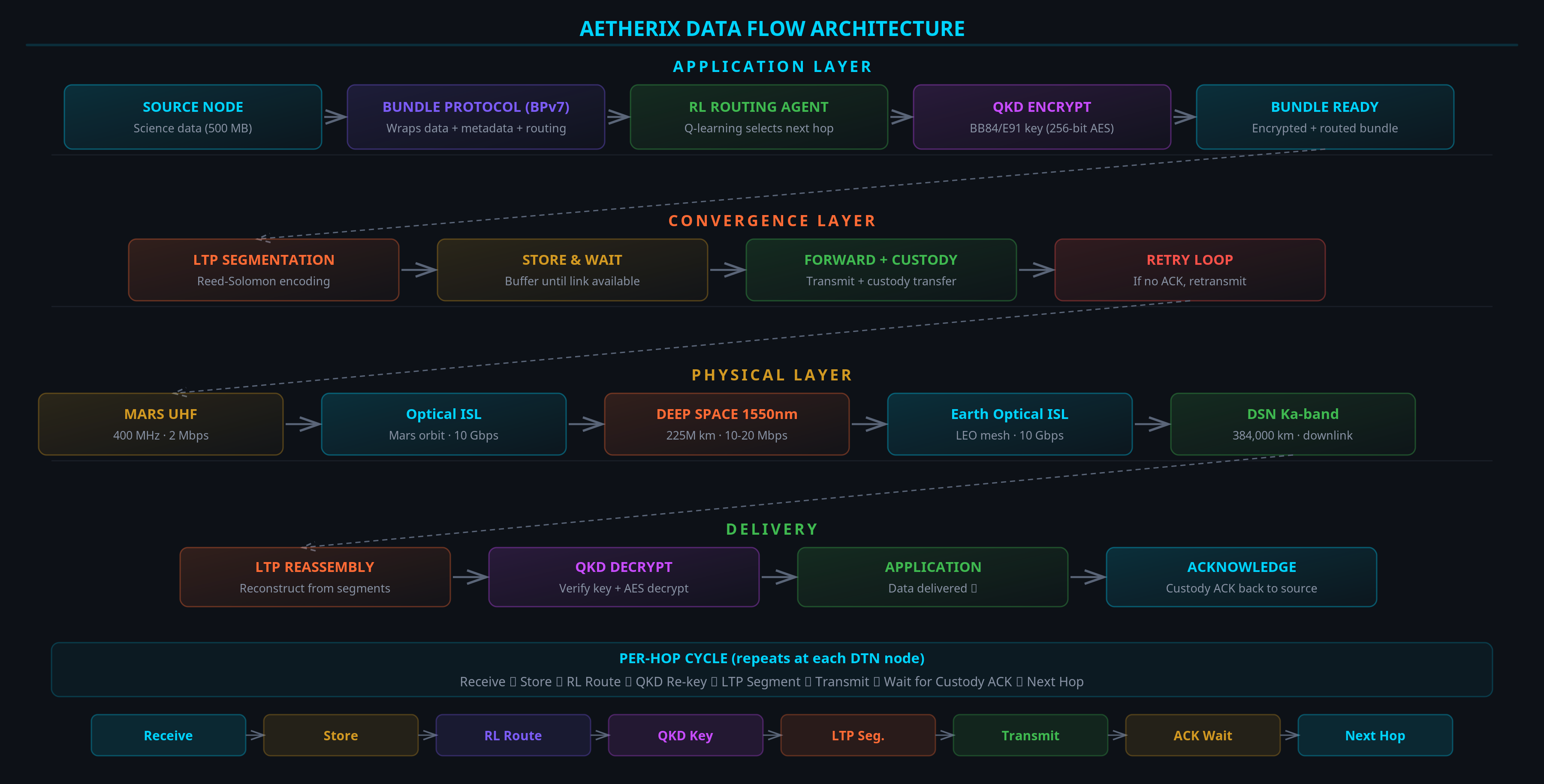
Instead of requiring an end-to-end connection, DTN breaks the journey into hops. At each hop, the data is stored safely until the next connection window opens.
Create
The sender packages data into a “bundle” with a destination address, priority level, and lifetime. Think of it as addressing a package with tracking information.
Store
The bundle waits at the current node until a communication link to the next hop becomes available. This could be minutes, hours, or even days — the data is safe.
Forward
When the link opens, the bundle is transmitted to the next node in the path. Each transmission is confirmed before the bundle moves on.
Custody Transfer
The receiving node takes legal “custody” of the bundle — it’s now responsible for safe delivery. If anything goes wrong, the data isn’t lost. It’s like registered mail with guaranteed delivery.
Deliver
Steps 2–4 repeat until the bundle reaches its final destination. The entire journey might take hours, but the data arrives intact and verified.
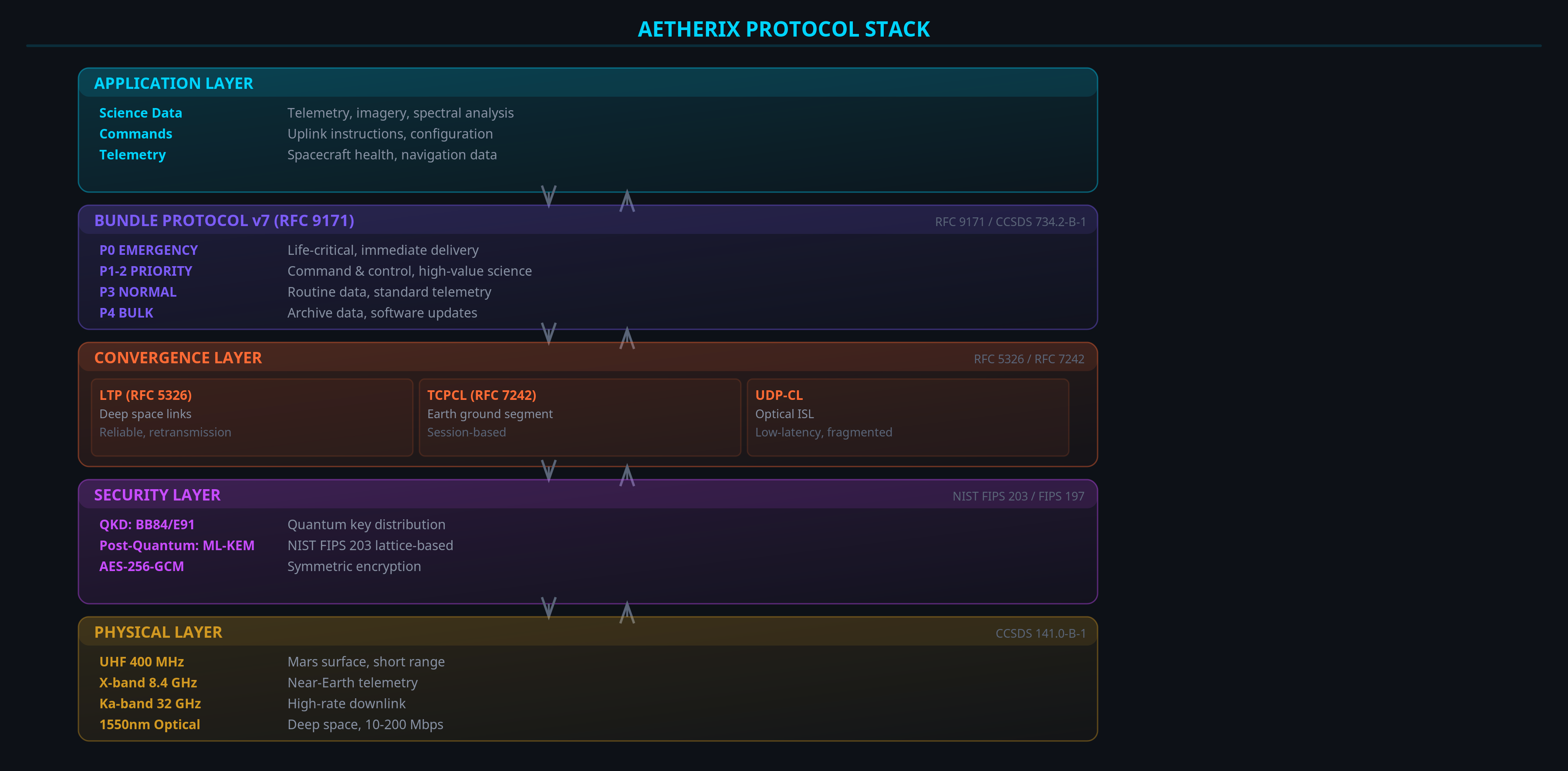
Not all data is equally urgent. BPv7 defines 5 priority classes so the network can make intelligent decisions about what to send first when bandwidth is limited.
Life-threatening alerts, abort commands. Must be delivered immediately — bypasses all other traffic. Think: “Solar flare incoming, take cover now.”
Telemetry, navigation updates, time-sensitive science data. Standard operational traffic — the majority of daily communications.
Software updates, archive dumps, high-res image batches. Can wait for off-peak windows — delivered when capacity allows.
Bundle Protocol v7 (BPv7) is the official IETF standard for delay-tolerant networking, developed jointly with CCSDS (the international body for space communications). It defines how bundles are created, addressed, routed, and delivered across challenged networks — from deep space to disaster zones.
How AETHERIX Works
Four key innovations working together to enable reliable, high-speed, quantum-secure communication between Earth and Mars.
Optical Link Budget
Laser Communications at 1550nm
Instead of radio waves, AETHERIX uses infrared lasers (1550nm wavelength) to beam data through space. This allows 10–100× higher data rates than traditional RF systems.
Reinforcement Learning Routing
AI That Learns the Best Path
Traditional space networks use fixed routing tables that must be manually updated. AETHERIX uses a reinforcement learning agent that learns from experience which paths work best.
Quantum Key Distribution
Unbreakable Encryption from Physics
AETHERIX uses quantum mechanics to securely distribute encryption keys. Any attempt to eavesdrop physically disturbs the quantum states, alerting both parties immediately.
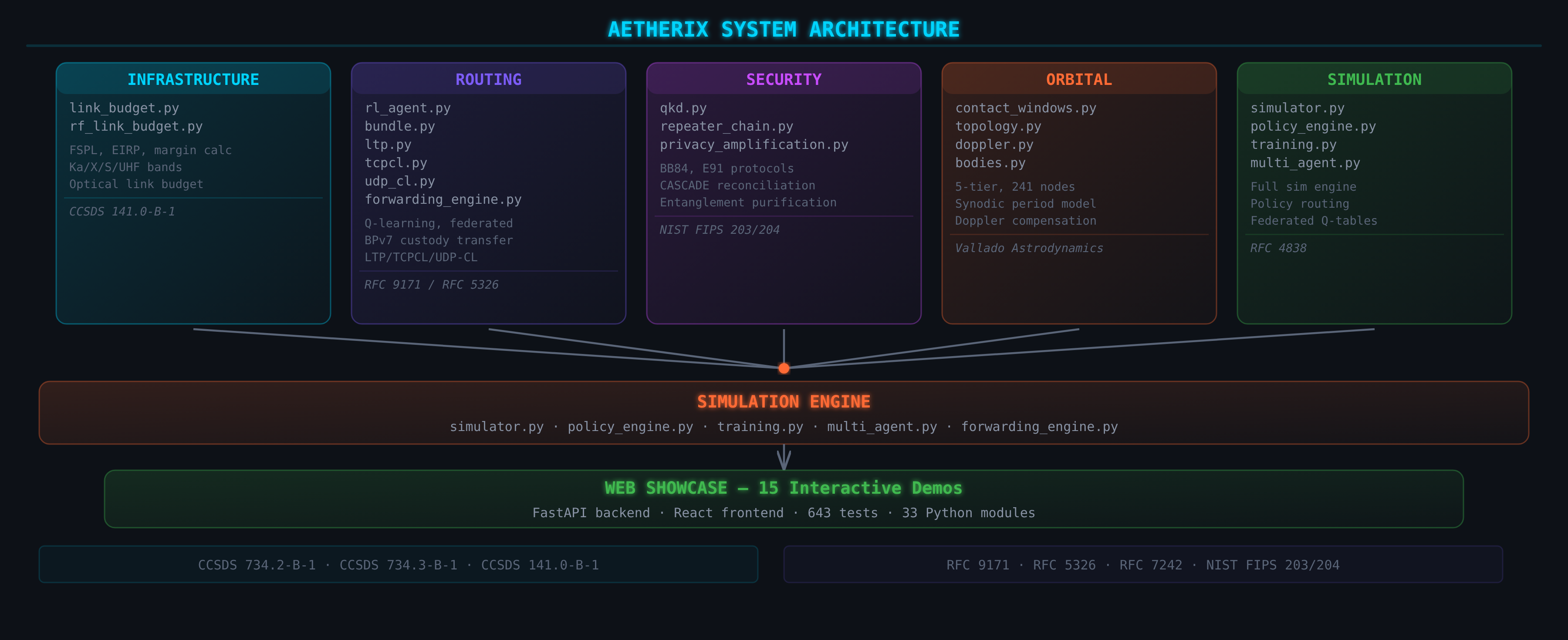
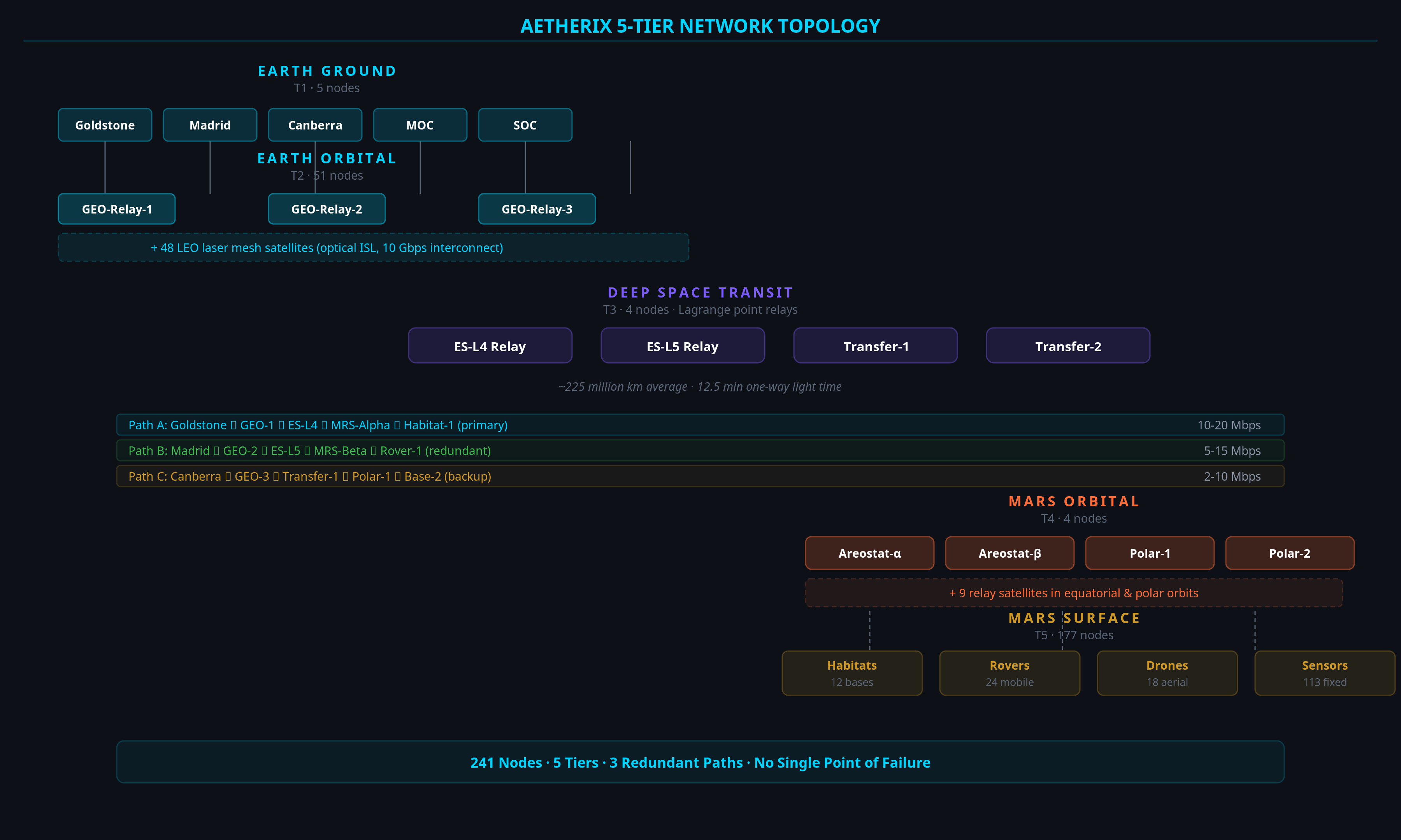
5-Tier Network Architecture
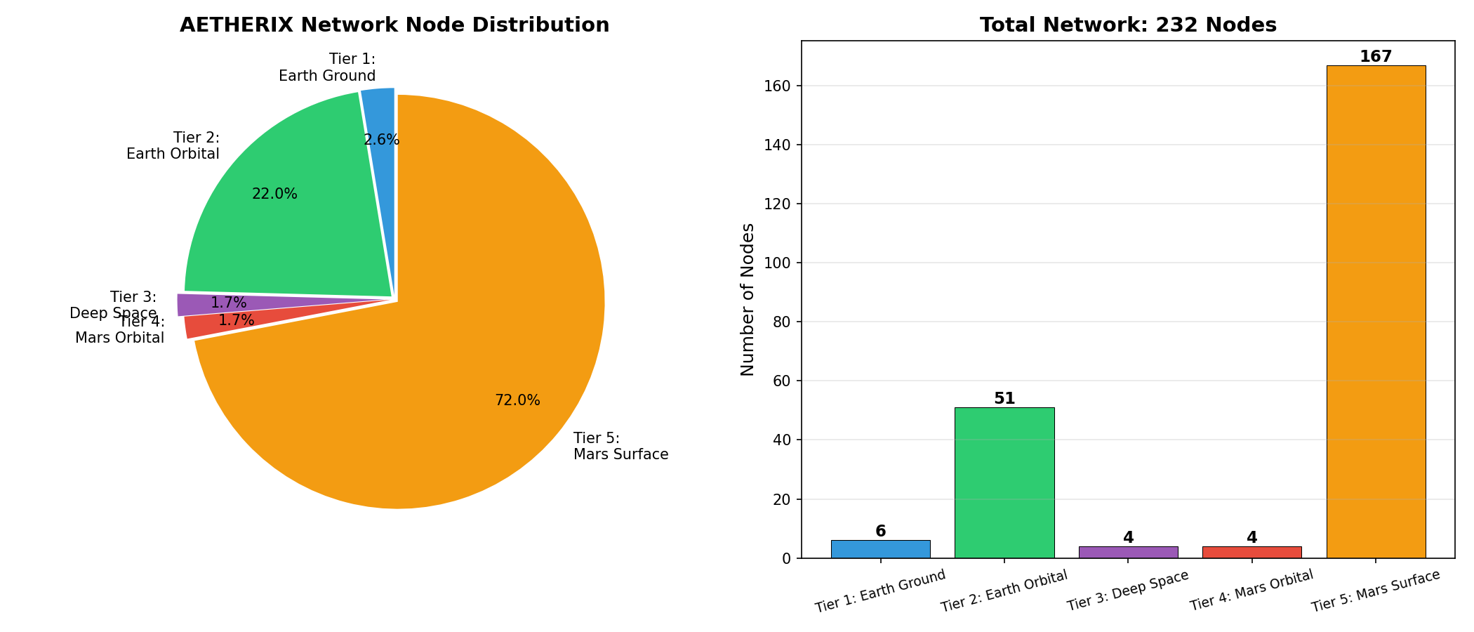
241 Nodes Across 5 Layers
The network spans from Earth’s surface to Mars’s surface through 5 distinct tiers, with relay satellites at Lagrange points maintaining connectivity even during solar conjunction blackouts.
Earth-segment links between ground stations and GEO relays. Reliable, ordered delivery over TCP — similar to how web browsers communicate, but carrying space bundles.
Deep-space links between Lagrange relays and Mars orbiters. Handles 3–22 minute delays with selective retransmission — only resend what was lost, not the whole bundle.
Inter-satellite laser links within constellations. Fragmented delivery with simulated packet loss — optimized for speed over the LEO and GEO laser mesh.
The Journey to Mars
Understanding the physics of Earth–Mars communication — distances, delays, orbital mechanics, and why timing is everything.
Signal delay: ~3 minutes one way. Data rates can reach 200 Mbps — comparable to home broadband. This is the golden window.
Signal delay: ~12.5 minutes one way. Data rates: 10–20 Mbps. This is the typical operating condition.
Signal delay: ~22 minutes one way. Data rates drop to 2–5 Mbps. And Mars is behind the Sun — direct communication is blocked.
Imagine you’re an astronaut on Mars and you send a message to Mission Control: “We found something interesting!”
- T+0 min You send the message from Mars
- T+12 min Message arrives at Earth (average distance)
- T+12 min Mission Control reads it and immediately replies: “Tell us more!”
- T+24 min You receive the reply. 25 minutes for a simple back-and-forth.
Earth orbits the Sun every 365.25 days. Mars takes 686.98 days. Because they move at different speeds, Earth “laps” Mars roughly every 780 days (the synodic period). This creates a repeating pattern:
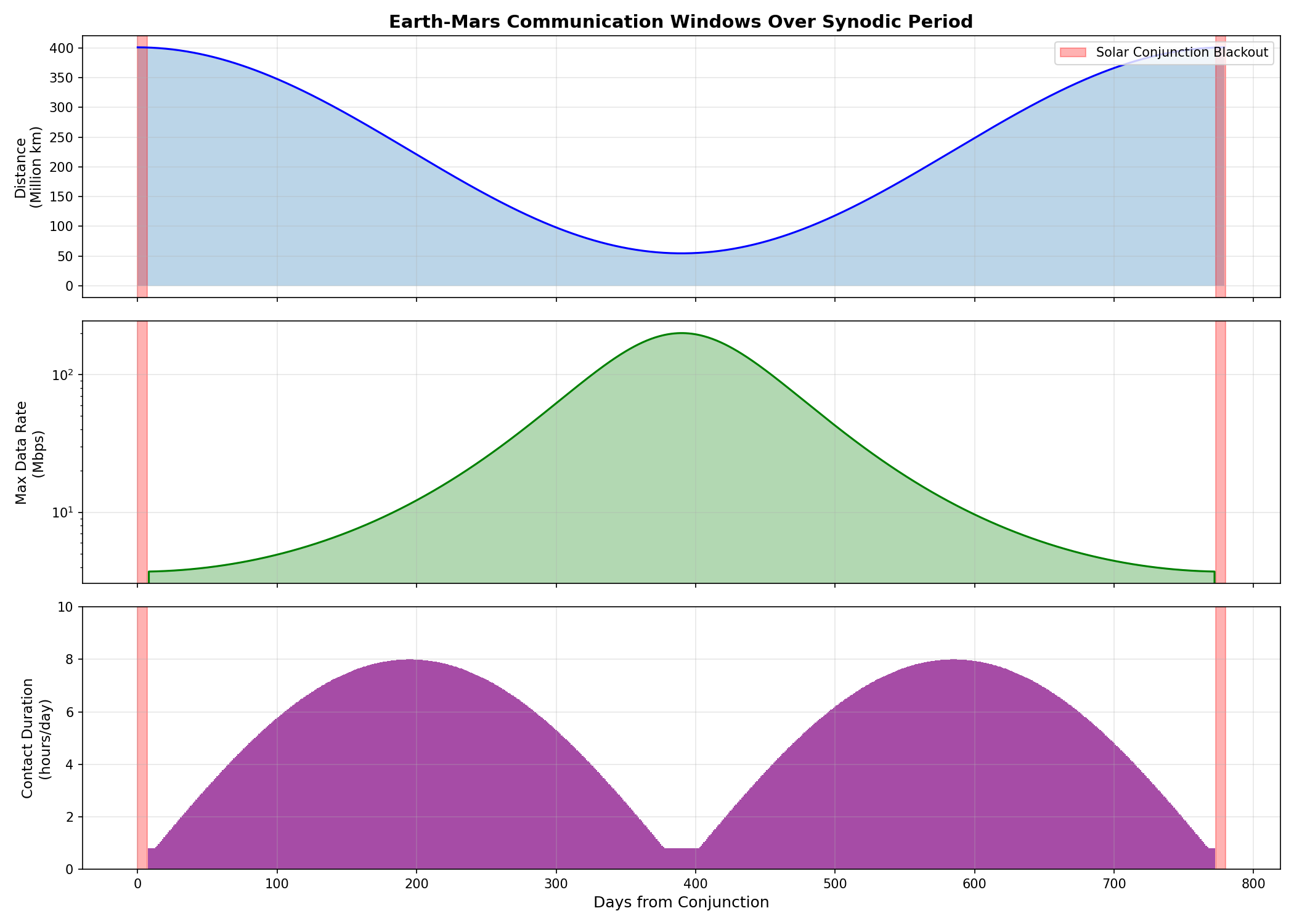
Communication isn’t available 24/7. Contact windows are scheduled periods when a ground station on Earth has line-of-sight to a Mars orbiter or relay:
The Network Architecture
A 5-tier, 241-node network spanning from Earth’s surface to Mars’s surface — with relay satellites at strategic points to maintain connectivity around the clock.
Earth Ground Stations
5 nodes — NASA’s Deep Space Network (DSN): Goldstone (California), Madrid (Spain), Canberra (Australia), plus the Mission Operations Center and Science Operations Center.
Earth Orbital Relays
51 nodes — 3 GEO relay satellites for continuous Earth coverage, plus 48 LEO satellites forming a laser inter-satellite mesh (similar to SpaceX Starlink, but for deep space backhaul).
Deep Space Transit
4 nodes — Relay satellites at Earth-Sun Lagrange points L4 and L5, plus 2 transfer orbit satellites. These are the critical “bridge” nodes between the Earth and Mars systems.
Mars Orbital Relays
4 nodes — 2 areostationary orbiters (Mars’ equivalent of geostationary satellites at 17,032 km altitude) providing continuous coverage of fixed surface locations, plus 2 polar orbiters for global coverage.
Mars Surface Assets
177 nodes — Human habitats, scientific bases, exploration rovers, reconnaissance drones, weather stations, and environmental sensors. These are the “endpoints” generating and consuming data.
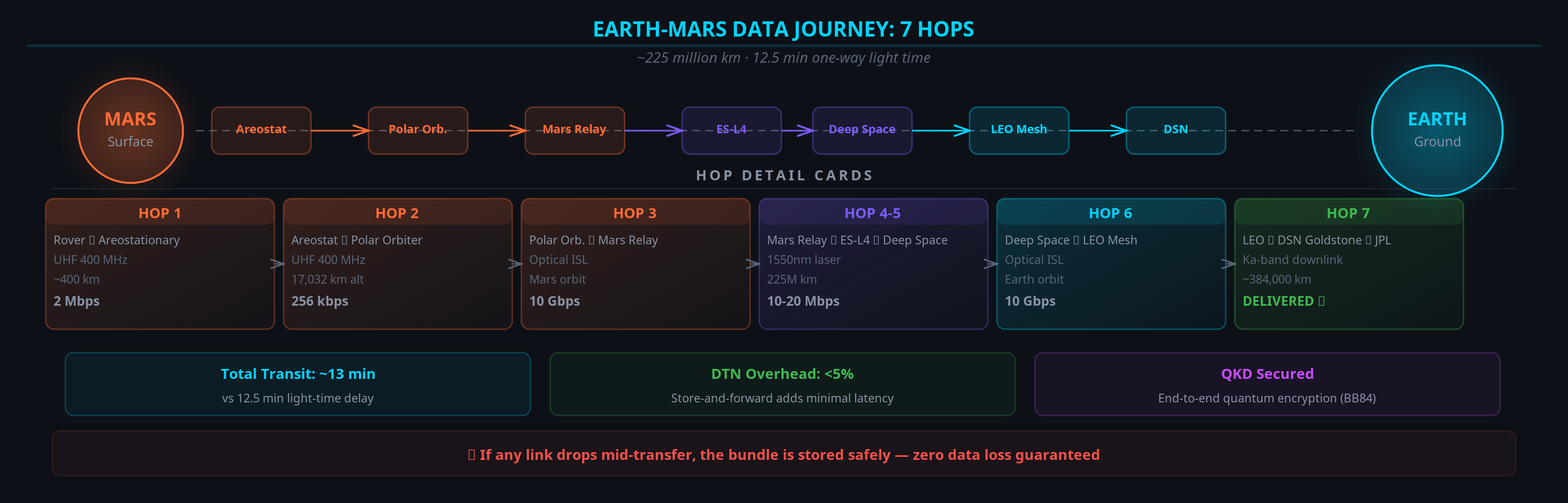
2. Bundle transmitted via UHF to areostationary orbiter (T5 → T4)
3. Orbiter forwards via optical laser to deep space relay (T4 → T3)
4. Deep space relay beams toward Earth’s LEO mesh (T3 → T2)
5. LEO mesh routes to the nearest DSN-capable satellite (T2 → T2)
6. Satellite downlinks to DSN ground station (T2 → T1)
7. Ground station delivers to Mission Control (T1 → T1)
Total: 7 hops, ~12.5 minutes (mostly light-time delay)
Altitude: 160–2,000 km. Orbital period: 90–120 minutes. Role: Rapid-response relay mesh.
AETHERIX deploys 48 LEO satellites in a Walker constellation at ≈550 km altitude (similar orbital shell to Starlink). Each satellite carries a 1550nm optical terminal for inter-satellite links (ISL) and a Ka-band transceiver for ground uplink.
Altitude: 35,786 km (exactly). Orbital period: 23h 56m 4s (matches Earth’s rotation). Role: Persistent relay over fixed ground stations.
AETHERIX uses 3 GEO relay satellites positioned over the Americas, Europe/Africa, and Asia/Pacific. Each GEO satellite maintains a permanent optical downlink to its regional DSN station and a Ka-band uplink to the LEO mesh.
NASA’s Deep Space Network is the backbone of all interplanetary communication. Three complexes spaced ≈120° apart ensure 24/7 coverage of the solar system.
35°N latitude. 70m + 34m antennas. Primary downlink for Mars missions. Houses the Signal Processing Center that demodulates deep-space signals as weak as 10−²¹ watts.
40°N latitude. 70m + 34m antennas. European node, provides overlap coverage with both Goldstone and Canberra during orbit shifts.
35°S latitude. 70m + 34m antennas. Southern hemisphere coverage essential for Mars observations during certain orbital geometries.
Lagrange points are positions in a two-body orbital system where a smaller object can maintain a stable position relative to the two larger bodies, balanced by their gravitational pulls.
A relay satellite here trails Earth by 60° (≈150M km ahead). It can see Mars even when Earth can’t — during solar conjunction, L4 has an unobstructed view of both planets from a different angle.
Trails Earth by 60° (≈150M km behind). Provides a second relay path independent of L4. If one relay fails, the other maintains service.
Mars’ equivalent of Earth’s geostationary satellites. The term comes from Ares (Greek name for Mars) + stationary.
Altitude: 17,032 km above Mars’ equator. Orbital period: 24h 37m (matches Mars’ sidereal rotation). A satellite at this altitude appears stationary from a fixed point on the Martian surface.
AETHERIX deploys 2 polar orbiters in sun-synchronous orbits around Mars at ≈300–400 km altitude, similar to Mars Reconnaissance Orbiter (MRO).
Role: Complement the areostationary orbiters by covering the Martian poles (which areostationary satellites cannot see from the equatorial plane) and providing redundant relay paths for high-latitude surface assets.
Space Security
Why interplanetary communication needs quantum-proof security, and how quantum physics provides an unbreakable solution.
- ✗ RSA — Used in most internet security (HTTPS, SSH)
- ✗ ECC — Elliptic curve cryptography
- ✗ Diffie-Hellman — Key exchange protocols
- ✓ Information-theoretic security — based on physics, not math
- ✓ Eavesdropper detection — any interception is immediately visible
- ✓ Future-proof — no computer can ever break the laws of physics
Quantum Transmission
Alice (Earth) sends a stream of photons, each representing a random bit (0 or 1) in a randomly chosen basis (rectilinear or diagonal). Think of it as sending letters in randomly chosen alphabets.
Measurement
Bob (Mars) measures each photon in a randomly chosen basis. When his basis matches Alice’s, he gets the correct bit. When it doesn’t, he gets a random result. About 50% of bases will match.
Sifting
Alice and Bob publicly compare which bases they used (not the actual bits). They keep only the bits where their bases matched. This is their “sifted key.”
Error Check (QBER)
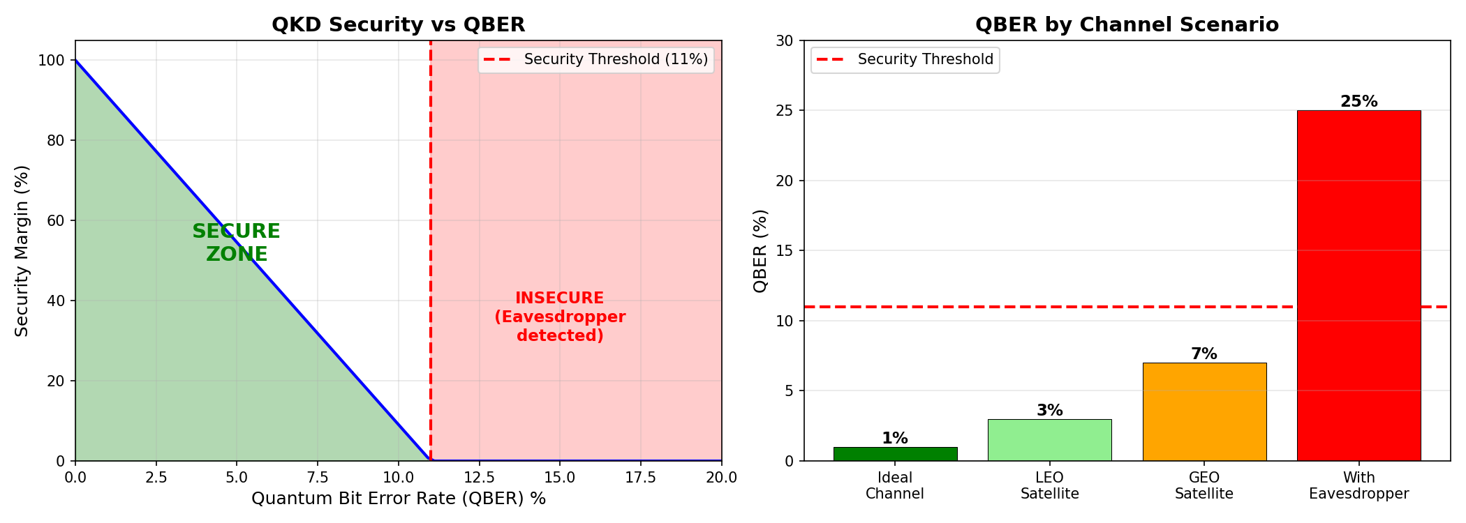
They compare a subset of the sifted key to calculate the Quantum Bit Error Rate (QBER). If QBER < 11%, no eavesdropper was detected. If QBER ≥ 11%, someone was listening — they abort and try again.
Privacy Amplification
They apply a mathematical function to the sifted key that compresses it, removing any partial information an eavesdropper might have gained. The result is a shared secret key that is provably secure.
The protocol uses two conjugate bases for encoding classical bits into quantum states:
Bit 0 → |0⟩ (vertical polarization). Bit 1 → |1⟩ (horizontal polarization). Measured with a vertical/horizontal polarizer.
Bit 0 → |+⟩ (+45° polarization). Bit 1 → |−⟩ (−45° polarization). Measured with a diagonal/anti-diagonal polarizer.
Protocol execution (N photons):
- Transmission: Alice generates N random bits and N random bases. For each bit i, she prepares photon i in the state |ψ⟩ corresponding to her random bit value in her random basis.
- Measurement: Bob independently chooses N random bases and measures each photon. If his basis matches Alice’s, he gets the correct bit with certainty. If it doesn’t match, quantum mechanics dictates he gets a random result (50/50 chance of either bit).
- Sifting (public channel): Alice and Bob publicly announce their basis choices (not the bit values). They discard all bits where bases didn’t match — roughly 50%. The remaining ≈N/2 bits form the sifted key.
- QBER estimation: They publicly compare a random subset (≈25%) of the sifted key to estimate the Quantum Bit Error Rate. In the absence of eavesdropping, QBER comes only from channel noise (typically 1–4%).
- Eavesdropper detection: If Eve intercepts and measures a photon, she must choose a basis. When she guesses wrong (≈50% of the time), her measurement disturbs the quantum state. This introduces a ≈25% error rate in the sifted key — well above the 11% security threshold.
- Privacy amplification: If QBER < 11%, Alice and Bob apply a universal hash function (e.g., based on Toeplitz matrices) to compress the sifted key. The result is a shorter key about which Eve has negligible information (<2⁻ⁿ⁸ bits).
QKD = Quantum Key Distribution. A family of protocols that use quantum mechanical phenomena (superposition, entanglement, measurement disturbance) to establish a shared secret key between two parties with information-theoretic security.
Security guarantee: Unlike classical key exchange (Diffie-Hellman, RSA), QKD’s security does not depend on computational assumptions. It is provably secure against an adversary with unlimited computing power, including quantum computers.
PQC = Post-Quantum Cryptography. Classical cryptographic algorithms designed to resist attacks by quantum computers. Unlike QKD (which uses physics), PQC relies on mathematical problems believed to be hard for both classical and quantum computers.
NIST Standards (2024):
- ✓ ML-KEM (FIPS 203) — Key encapsulation, based on CRYSTALS-Kyber. Replaces RSA key exchange.
- ✓ ML-DSA (FIPS 204) — Digital signatures, based on CRYSTALS-Dilithium. Replaces RSA/ECDSA signatures.
- ✓ SLH-DSA (FIPS 205) — Hash-based signatures. Backup with minimal security assumptions.
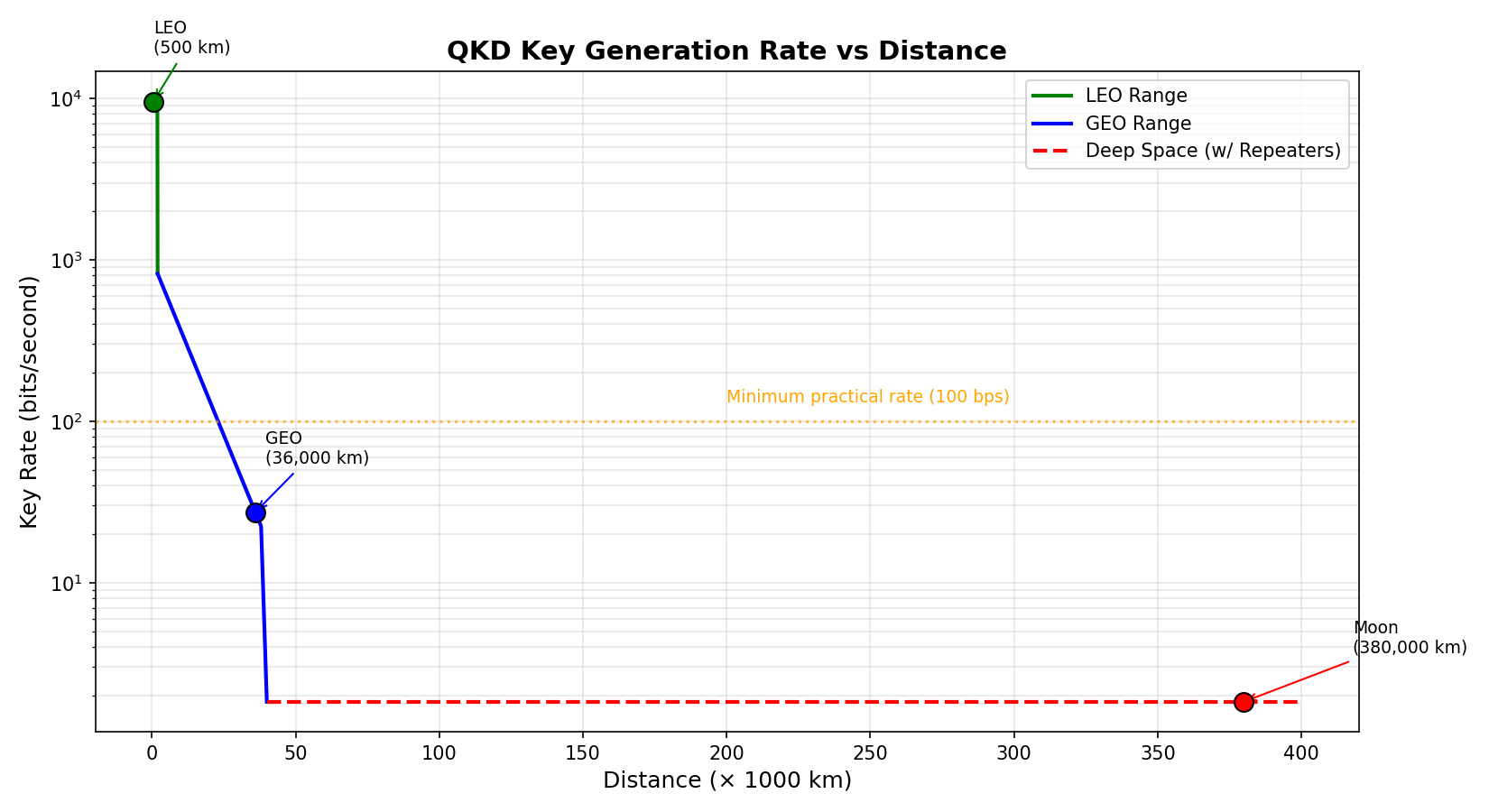
Satellite-to-ground QKD (similar to China’s Micius satellite). Proven technology. Range: 500–2,000 km.
ProvenEntanglement-based QKD (E91) with higher photon loss at 36,000 km. Requires quantum repeaters at LEO.
Near-termQuantum repeaters at Lagrange points enable entanglement swapping across 225M km. Low rate but provably secure.
FutureBB84, Step by Step
Forget “Alice sends quantum states.” Picture two people passing single photons whose polarization can be measured in two different ways — and an eavesdropper who physically cannot look without leaving fingerprints. This page walks the whole protocol with real numbers, then lets you run it.
A basis is really just the question you ask the photon. There are two questions, and each one has two possible answers — so each photon can carry one bit, encoded four possible ways.
vertical, 0°
horizontal, 90°
diagonal, +45°
diagonal, −45°
Alice generates a random bit and a random basis for each photon. She does not send her bits — she sends the polarizations those bits encode.
| Photon | Alice’s bit | Alice’s basis | Photon sent | Meaning |
|---|---|---|---|---|
| 1 | 1 | Z | ─ | horizontal |
| 2 | 0 | X | ↗ | +45° |
| 3 | 1 | X | ↘ | −45° |
| 4 | 0 | Z | │ | vertical |
| 5 | 1 | Z | ─ | horizontal |
| 6 | 0 | X | ↗ | +45° |
| 7 | 1 | Z | ─ | horizontal |
| 8 | 1 | X | ↘ | −45° |
Bob has no idea what Alice chose, so he flips his own coin for each arriving photon. Three cases show what happens:
Alice sent bit 1 in Z (─). Bob measures in Z.
He asked the question the photon was built to answer, so he gets 1, with certainty.
Alice sent bit 0 in X (↗). Bob measures in Z.
A +45° photon is neither vertical nor horizontal, so the answer is a coin flip — 0 or 1, 50/50. Crucially, nothing in the result tells Bob he guessed wrong.
Alice sent bit 1 in X (↘). Bob measures in X.
Right question again — he gets 1. Note that “right basis” has nothing to do with Z vs X; it only means the same as Alice’s.
Running all eight, Bob might record:
Some of these are Alice’s bits; some are noise from a wrong-basis guess. Bob cannot tell which is which — and that is fine, because the next step sorts it out without either of them revealing a single bit.
Now they talk over an ordinary, completely public channel. Alice says “my bases were Z X X Z Z X Z X.” Bob says “mine were Z Z X X Z X X Z.” Neither of them says a single bit value. Announcing a basis leaks nothing: knowing Alice asked the Z question tells you nothing about whether her answer was 0 or 1.
| Photon | Alice | Bob | Agree? | Alice’s bit | Bob’s bit | Verdict |
|---|---|---|---|---|---|---|
| 1 | Z | Z | ✓ | 1 | 1 | KEEP |
| 2 | X | Z | ✗ | 0 | 1 | discard |
| 3 | X | X | ✓ | 1 | 1 | KEEP |
| 4 | Z | X | ✗ | 0 | 1 | discard |
| 5 | Z | Z | ✓ | 1 | 1 | KEEP |
| 6 | X | X | ✓ | 0 | 0 | KEEP |
| 7 | Z | X | ✗ | 1 | 0 | discard |
| 8 | X | Z | ✗ | 1 | 1 | discard |
Alice has
Bob has
🎉 A shared secret string, and nothing that would let a listener reconstruct it was ever spoken aloud.
Half the photons are wasted — and that is by design, not inefficiency. Because Alice and Bob each pick between two bases independently, they agree about 50% of the time. That ½ sifting factor is the q in the key-rate formula further down.
Everything above, running top to bottom. Photons fall from Alice through the quantum channel to Bob; below Bob the picture switches from photons to bits, because that is exactly where the physics hands over to classical information theory. Turn Eve on and watch the QBER climb toward 25%.
Loading simulator…
Eve sits on the channel and runs the obvious attack: intercept, measure, resend. Follow one photon through it.
This is the part that usually makes BB84 click. Look only at the bits that survive sifting — the ones where Alice and Bob agreed on a basis. For such a bit to come out wrong, two independent coin flips both have to go badly:
Alice and Bob don’t compare the whole sifted key — that would burn all of it. They publicly reveal a randomly chosen subset: “let’s compare positions 7, 19, 31, 44…”
Those 100 bits are now public knowledge, so they are discarded — the sample is spent, not free. The random choice of positions matters: it stops Eve from concentrating her attack where she knows nobody will look.
A relatively clean channel. About 72% of the sifted bits survive into the final key.
Still workable, but expensive: only about 27% survives. Same protocol, far less key.
Under standard BB84 assumptions, no secure key can be extracted at all. Abort.
Even with no Eve at all, detectors misfire and photons scatter. Alice and Bob’s sifted keys will differ in a few places, and a key that differs in even one bit is useless.
So they run information reconciliation (CASCADE, or an LDPC code) over the public channel — exchanging parities until the keys match.
Now Alice and Bob hold identical keys — say 600 bits — but they must assume Eve holds partial information about them, both from the channel and from the reconciliation chatter.
They do not try to work out which bits she knows. They can’t, and they don’t need to. Instead they compress: run the whole string through a universal hash function and keep a shorter output.
The intuition: “even if Eve knew a chunk of our 600-bit string, she should know essentially nothing about this shorter one.” Compression converts partial knowledge into no knowledge — at the price of key length. That is why the final key is always meaningfully shorter than the sifted key, even on a perfect channel.
single photons
1,000 × ½ — bases agree half the time
not 485 — see below
key = ½ × N × (1 − QBER) × f(EC) and get 500 × 0.97 ≈ 485 bits. That treats the 3% purely as bits to be repaired. But the errors are not just damage — they are evidence of how much Eve might know, and that has to be paid for twice: once in the reconciliation leak, once in privacy amplification.| Term | Meaning | Value here |
|---|---|---|
| q | sifting factor — fraction of photons where the bases agree | ½ |
| Q | measured quantum bit error rate | 0.03 |
| h₂(Q) | binary entropy — −Q log₂Q − (1−Q) log₂(1−Q) | 0.194 |
| 1 − 2h₂(Q) | fraction of the sifted key that survives EC + PA | 0.611 |
| R | secret bits per photon sent | 0.306 |
So 1,000 transmitted single photons at 3% QBER yield roughly 306 secret bits — about 63% of the naive 485, and that is still an idealised figure before finite-key statistics, multi-photon pulses, detector dark counts and imperfect reconciliation efficiency take their cut.
The simulator above computes its key length with exactly this expression — drag the noise slider and watch how quickly the final key falls away as Q rises.
Optical Communications in Deep Space
How infrared lasers deliver 10–100× faster data rates than radio for interplanetary communication — and why pointing a beam at a target 400 million kilometers away is harder than it sounds.
Radio antennas spread their signal across a wide cone — like a floodlight. Optical lasers concentrate energy into a tight beam — like a laser pointer. At 1550 nm (infrared), the wavelength is 10,000× shorter than Ka-band radio, so the beam stays concentrated over interplanetary distances.
Ka-band RF: ~0.5 mrad → spot size ~200,000 km at Mars distance
The optical beam is 100× narrower, concentrating 10,000× more energy on the receiver.
Data rate scales with frequency. Optical at 193 THz (1550nm) can modulate information far faster than Ka-band at 26.5 GHz. The theoretical Shannon limit for optical is orders of magnitude higher than RF.
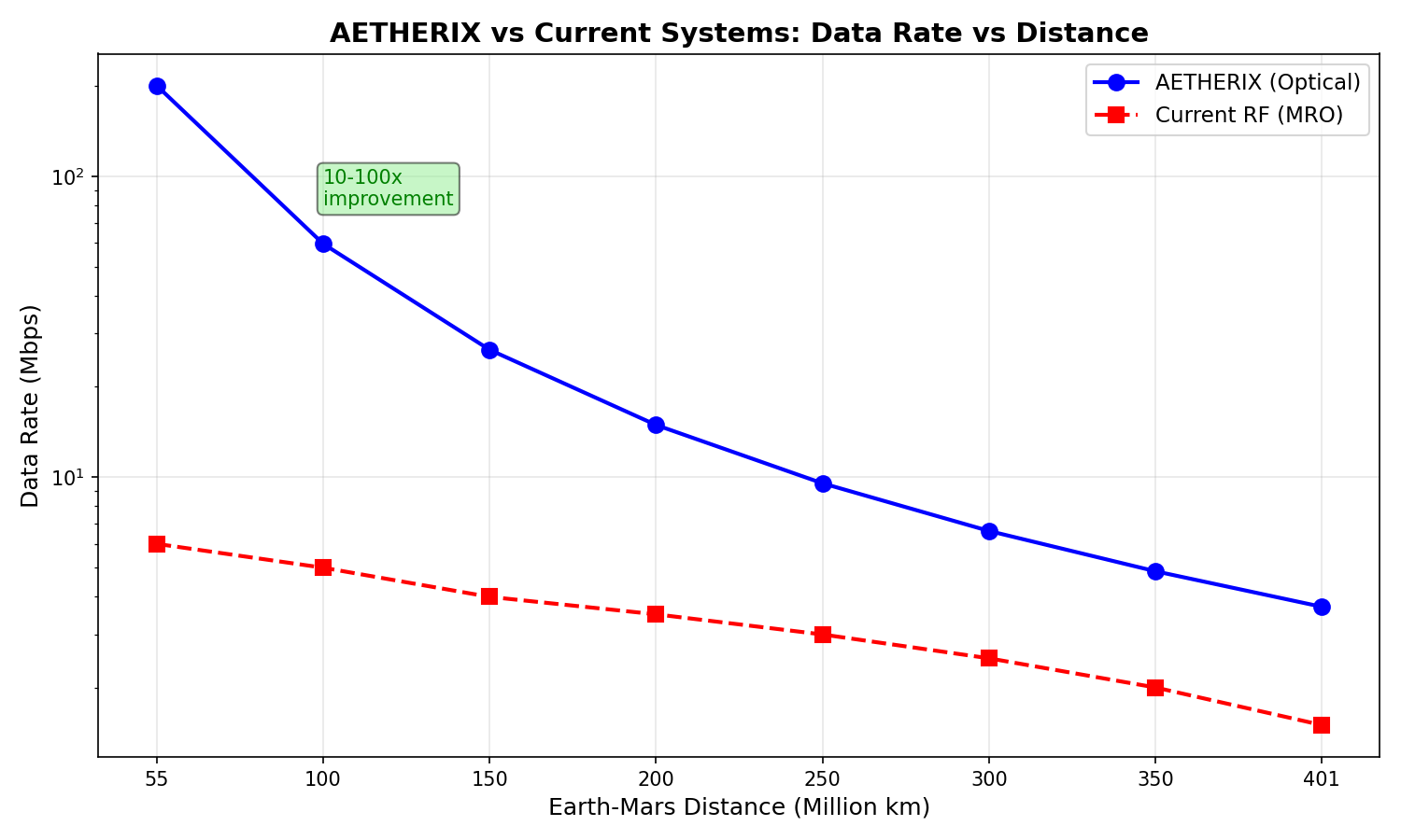
DSOC / AETHERIX (Optical): 2–200 Mbps (distance-dependent)
At opposition (55M km), optical can achieve 200 Mbps — enough for streaming HD video from Mars.
Optical signals can’t penetrate clouds. This is why AETHERIX uses hybrid optical/RF — when clouds block the laser at a DSN site, the system falls back to Ka-band radio. Sites like Goldstone (California desert) were chosen for their clear skies.
A 5 μrad beam at 225M km produces a ~1,100 km spot. The receiver must be within that spot. Spacecraft vibration, thermal deformation, and orbital motion all affect pointing. Requires sub-microradian pointing stability — achieved with fine-steering mirrors.
The Sun is an intense infrared source. When Mars is near solar conjunction, sunlight swamps the optical receiver. This creates the same ~2-week blackout as RF, but the effect is more severe for optical. Lagrange-point relays help maintain partial connectivity.
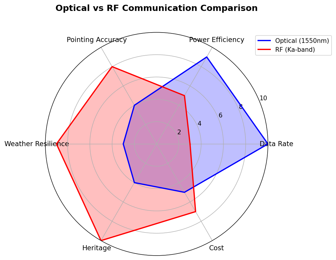
| Property | Optical (1550nm) | Ka-band (26.5 GHz) | X-band (8.4 GHz) |
|---|---|---|---|
| Wavelength | 1550 nm | 11.3 mm | 35.7 mm |
| Frequency | 193 THz | 26.5 GHz | 8.4 GHz |
| Beam Divergence | ~5 μrad | ~0.5 mrad | ~1.5 mrad |
| Max Data Rate | 200 Mbps | 50 Mbps | 6 Mbps |
| Weather Immunity | Low (clouds block) | Moderate (rain fade) | High |
| Power Efficiency | Very high | Moderate | Moderate |
| Best For | Bulk science downlink | High-rate backup | Reliable command/telemetry |
| Heritage | DSOC (2023) | MRO, Mars Express | Viking, MGS, MRO |
DSOC — Deep Space Optical Communications
NASA has already flown the thing AETHERIX models. DSOC is the technology demonstration that took laser communications out of Earth orbit and into deep space — and it is the flight heritage that makes the optical choice defensible rather than speculative.
DSOC is a NASA technology demonstration riding aboard the Psyche spacecraft, which launched on 5 October 2023 toward the metal-rich asteroid of the same name. Psyche is the mission; DSOC is a passenger on it, proving a communications technology while the spacecraft goes about its own science.
That distinction matters: DSOC is not a communications mission. It is a risk-reduction experiment flown alongside a conventional radio link, so that if the laser had failed, nothing would have been lost. NASA did not bet a mission on it — and neither does AETHERIX, which is why the architecture keeps Ka-band RF as a fallback.
A radio wave at Ka-band has a wavelength of roughly 1 cm. An infrared laser at 1550 nm has a wavelength about 10,000× shorter. Beam divergence scales with wavelength over aperture, so for the same size telescope the laser beam spreads far less — more of the transmitted energy lands on the receiver instead of spilling into empty space.
That is the entire argument in one sentence: shorter wavelength, tighter beam, more photons on target. NASA measured the result at at least 10× the data rate of state-of-the-art radio systems of comparable size and power.
Streamed an ultra-high-definition video to Earth from 31 million km (19 million miles) at the system’s maximum bitrate of 267 Mbps.
Downlinked Psyche data from 494 million km (307 million miles) — further than the maximum Earth–Mars distance of 401 million km.
Data rates at least ten times higher than state-of-the-art radio telecommunications systems of comparable size and power.
A flight laser transceiver transmitting near-infrared photons at 1550 nm through a 22 cm aperture telescope, driven by a 4 W laser. It also carries a photon-counting camera to receive the low-rate uplink.
A powerful modulated laser at the Optical Communication Telescope Laboratory (OCTL), part of JPL’s Table Mountain Facility near Wrightwood, California. The uplink doubles as a beacon the spacecraft locks onto for pointing.
A superconducting nanowire photon-counting receiver at Caltech’s Palomar Observatory in San Diego County. Not a conventional radio dish — a detector cold enough to register individual photons.
On a terrestrial fibre link the receiver measures a waveform — there is so much light that you can treat it as a continuous signal. At interplanetary distance that is no longer true. Free-space path loss is around −353 dB at Mars opposition, so what arrives is not a waveform but a sparse trickle of individual photons, sometimes fewer than one per transmitted bit.
That is why the receiver is a superconducting nanowire single-photon detector cooled to a few kelvin: at that temperature a single arriving photon deposits enough energy to break superconductivity and produce a measurable voltage pulse. The information is carried in which time slot the photon arrives in — pulse-position modulation — rather than in amplitude.
| Parameter | DSOC (flown) | AETHERIX (modelled) | Comment |
|---|---|---|---|
| Wavelength | 1550 nm | 1550 nm | Identical — telecom heritage |
| Flight aperture | 22 cm | 22 cm | Identical |
| Laser power | 4 W | 5 W | Same class |
| Ground receive | Palomar (5.1 m) | 5 m Hale-class | Same class |
| Detector | SNSPD photon counting | Photon-counting model | Same physics |
| Coding | Coded (SCPPM) | Uncoded | The one real difference — ~13 dB |
So is the trade speed or volume? Neither, separately. Volume is just rate multiplied by how long the link is open — the same quantity seen over time. The real trade is data rate per kilogram and per watt, bought at the cost of availability. Here is that trade in the project’s own numbers, all at 225 million km and 2 Mbps:
| Configuration | Margin | Optical advantage | ≈ rate ratio |
|---|---|---|---|
| Optical — 5 W, 22 cm flight, 5 m ground | −7.92 dB | — | baseline |
| Ka-band, same 5 W / 22 cm / 5 m | −62.00 dB | +54.1 dB | ~255,000× |
| Ka-band, 34 m DSN dish, 5 W | −45.35 dB | +37.4 dB | ~5,500× |
| Ka-band, 34 m DSN dish, 100 W, 3 m spacecraft antenna | −9.65 dB | +1.7 dB | ~1.5× |
| Ka-band, 70 m DSN dish, 100 W, 3 m antenna | −3.37 dB | −4.6 dB | RF wins |
Rate for the same mass and power. Beam divergence scales as wavelength ÷ aperture, and 1550 nm is ~10,000× shorter than Ka-band, so far less energy is wasted spilling past the receiver. For a mission where every kilogram is contested, this is the decisive argument.
Availability. Cloud stops an optical link dead; Ka-band passes straight through. The tight beam also demands far harder pointing. So optical maximises rate, RF maximises uptime — and since volume = rate × uptime, neither wins volume outright.
If NASA has already flown deep-space laser comms, what is left to contribute? This is the sharpest challenge to the whole project, and it has a clean answer: DSOC solved a link problem. AETHERIX addresses a network problem.
DSOC connects one spacecraft to one ground station when both are in view. It has no routing, no relaying, no store-and-forward, and no notion of a bundle. It does not answer “what happens to this data when nobody is in view?” — which is the question DTN exists for.
Optical links do not penetrate cloud. A single ground site is weather-limited, which is why AETHERIX keeps Ka-band RF as a fallback and spreads receivers across sites. NASA made the same call: DSOC flew alongside Psyche’s conventional radio link, not instead of it.
When the Sun sits between Earth and Mars, the corona blocks the direct line of sight regardless of how good the laser is. That is a geometry problem, not a link-budget one — and it is why AETHERIX puts relays at the ES-L4 and ES-L5 Lagrange points.
The tighter beam that makes optical fast also makes it hard to aim. At 494 million km the spacecraft must point not at where Earth is, but at where Earth will be when the photons arrive — minutes of lead angle. Losing lock loses the link entirely.
Deep Space Communication Standards
The international standards that make interplanetary networking possible — from the IETF’s Bundle Protocol to CCSDS’s space link specifications.
Creates the internet standards (RFCs) that DTN builds on. Key RFCs include RFC 9171 (Bundle Protocol v7), RFC 5326 (LTP), RFC 4838 (DTN Architecture), and RFC 7242 (TCPCL). Open, community-driven process.
The space agency consortium (NASA, ESA, JAXA, CSA, etc.) that defines space-specific protocols. CCSDS 734.2-B-1 is the CCSDS Bundle Protocol (space profile of RFC 9171 BPv7); RFC 4838 defines the DTN architecture; CCSDS 734.3-B-1 (SABR) standardises contact-graph routing; CCSDS 141.0-B-1 covers optical links.
Defines cryptographic standards. For AETHERIX, the key standards are FIPS 203 (ML-KEM / CRYSTALS-Kyber for key encapsulation) and FIPS 204 (ML-DSA / CRYSTALS-Dilithium for digital signatures) — the new post-quantum cryptography standards finalized in 2024.
| Layer | Protocol | Standard | Purpose |
|---|---|---|---|
| Application | Bundle Protocol v7 | RFC 9171 / CCSDS 734.2-B-1 | End-to-end messaging with custody transfer |
| Transport | LTP (Licklider) | RFC 5326 | Reliable segmentation over long-delay links |
| Transport | TCPCL | RFC 7242 | TCP convergence layer for Earth segment |
| Transport | UDPCL | RFC 7122 | UDP convergence for optical inter-satellite links |
| Network | Contact Graph Routing (SABR) | CCSDS 734.3-B-1 | Static routing based on contact schedules |
| Network | RL Routing (AETHERIX) | Research | Adaptive routing via reinforcement learning |
| Security | BPSec | RFC 9172 | Bundle security (integrity + confidentiality) |
| Physical | Optical (1550nm) | CCSDS 141.0-B-1 | Laser communication physical layer |
| Physical | RF (Ka/X/S/UHF) | CCSDS 401.0-B-30 | Radio frequency physical layer |
TCP Convergence Layer. Used on Earth where TCP works — between DSN ground stations and mission control, between data centers. Reliable, ordered delivery. Segments bundles into TCP-friendly frames.
Licklider Transmission Protocol. The deep-space workhorse. Designed for links with 3–22 minute delays. Segments data, selectively retransmits only lost segments (not the whole payload). Report-based ACK instead of per-packet ACK.
UDP Convergence Layer. Used for high-speed optical inter-satellite links where reliability is handled by LTP above. Fire-and-forget with optional fragmentation. Best for LEO mesh laser links with low latency.
The Science Behind Quantum Key Distribution
How the fundamental laws of quantum physics — superposition, entanglement, and the no-cloning theorem — enable encryption that is provably unbreakable.
A quantum bit (qubit) doesn’t have a definite value until you measure it. Think of a coin spinning in the air — it’s neither heads nor tails until it lands. In BB84, Alice encodes bits in the polarization of photons. A photon polarized at 45° is in a superposition of horizontal (0) and vertical (1).
It is physically impossible to make an identical copy of an unknown quantum state. This is the mathematical proof (Wootters & Zurek, 1982) that makes QKD secure. Eve cannot intercept a photon, copy it, and send the original on to Bob — the universe forbids it.
Measuring a quantum system changes it irreversibly (wavefunction collapse). When Eve measures a photon in the wrong basis, she gets a random result — and the photon’s original state is destroyed. Bob’s subsequent measurement will disagree with Alice’s, revealing Eve’s presence as an elevated QBER.
Named after Charles Bennett and Gilles Brassard (1984). Alice prepares photons in specific states and Bob measures them. Simpler to implement. Used by China’s Micius satellite (2016) for the first satellite-to-ground QKD. Security relies on the no-cloning theorem.
Named after Artur Ekert (1991). A source creates entangled photon pairs — sending one to Alice and one to Bob. Their measurements are correlated even across vast distances (Einstein’s “spooky action at a distance”). Security is verified via Bell inequality violations — if the inequality holds, no eavesdropper is present.
Reinforcement Learning for Space Routing
How an AI agent learns to route data through the interplanetary network by trial and error — discovering strategies that outperform traditional static routing tables.
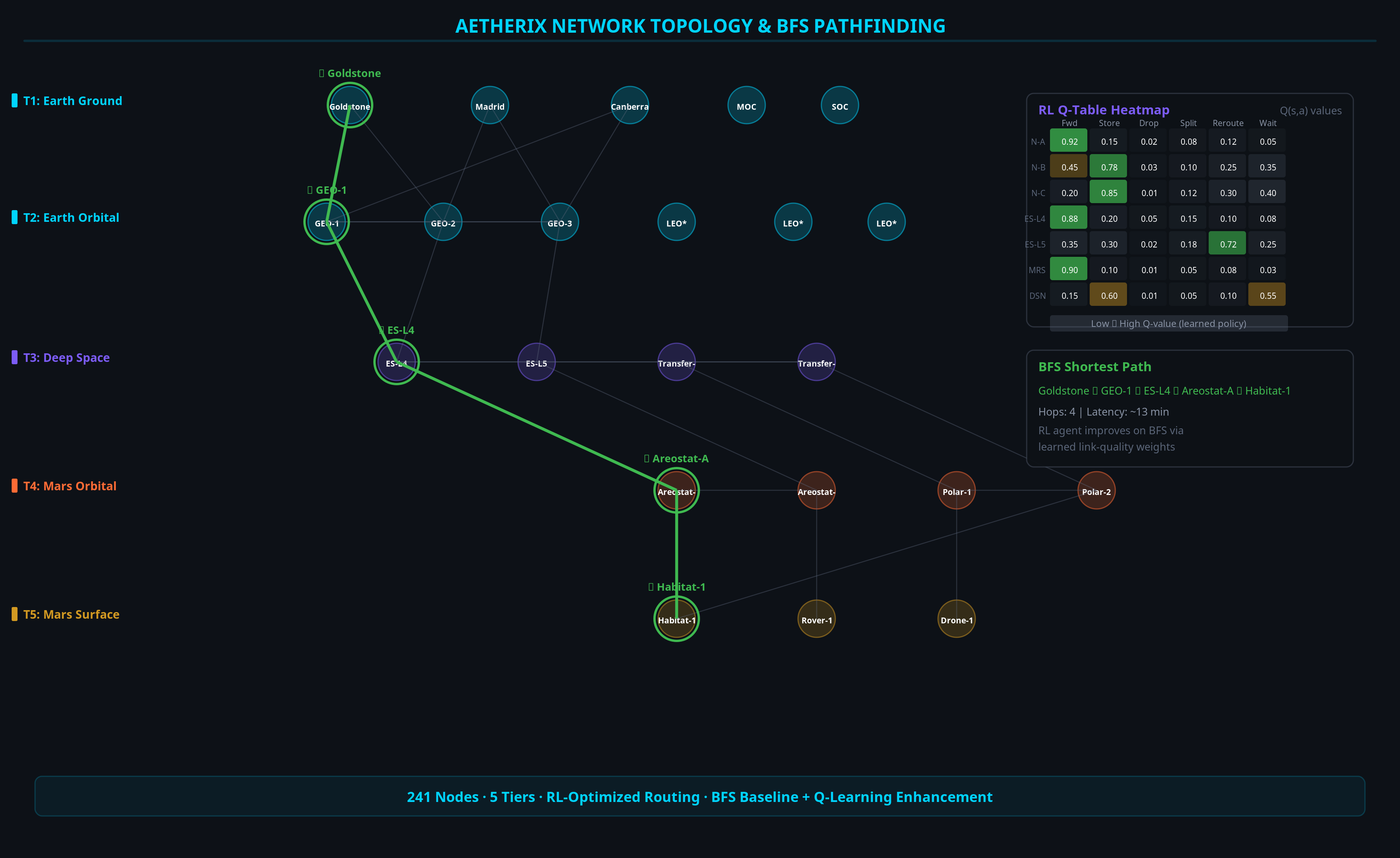
The agent observes the network state (current node, neighbors, link quality, buffer occupancy), chooses an action (forward to neighbor X, store, drop, or split), and receives a reward based on the outcome:
High reward for fast delivery to the correct destination. Penalty for delays, extra hops, dropped bundles, and wasted energy. The agent maximizes cumulative reward over time.
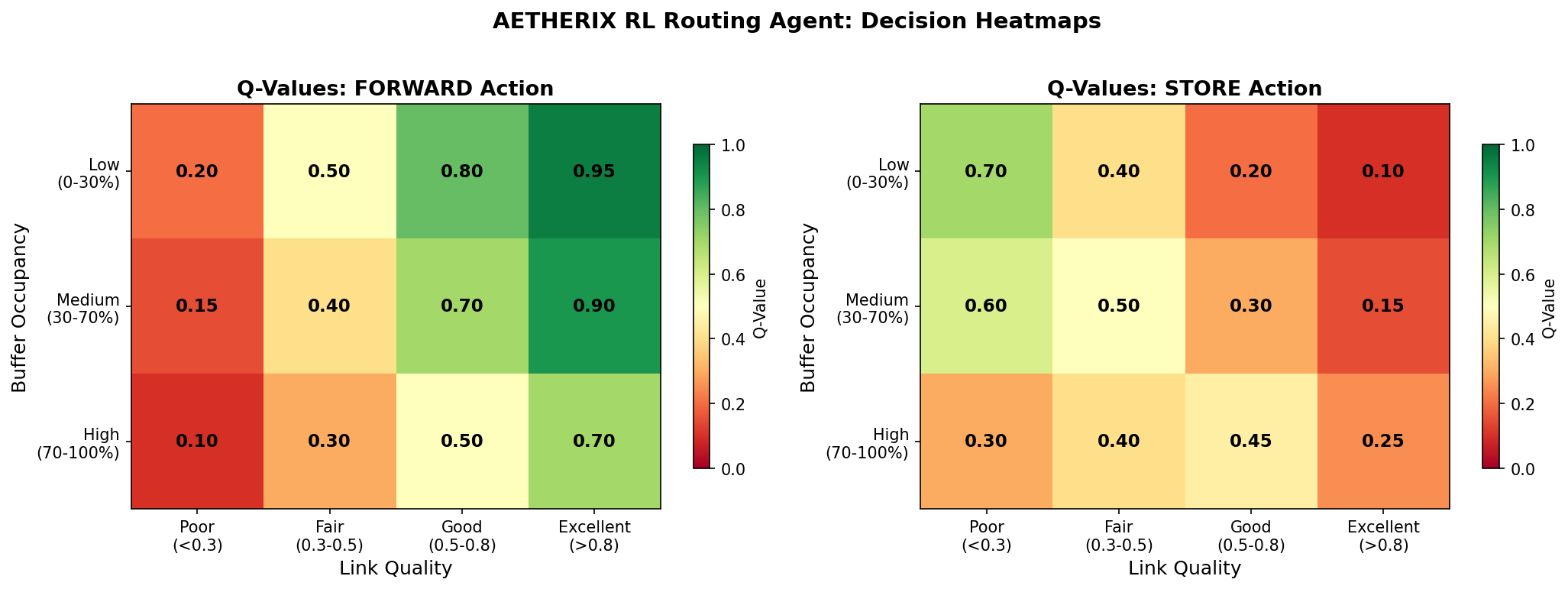
The agent maintains a Q-table — a lookup table that maps every (state, action) pair to an expected reward. After thousands of simulated routing decisions, the Q-table encodes the best action for every situation the agent has encountered. A high Q-value means “I’ve learned this action works well in this state.”
The agent tries random actions, including bad ones. This is essential — without exploration, the agent might never discover that a non-obvious route (through a Lagrange relay during conjunction) is actually the best strategy. Too much exploration wastes time on known-bad choices.
The agent uses its Q-table to pick the best-known action. This is efficient — it takes the routes it has already learned work well. But without occasional exploration, it can’t adapt when network conditions change (e.g., a node fails or a new link becomes available).
In the real network, every node runs its own RL agent — each one learning from local observations. The challenge: a single agent at one node only sees a small part of the network. Multi-agent federated learning solves this by periodically aggregating Q-tables across nodes:
Conjunction-proof rounds: federation aggregates over whichever agents are present — relays vanish for hours behind the Sun, so rounds never block on a straggler. And sync ships sparse Q-table deltas (only changed cells, as priority-class control traffic) instead of full tables — a round-trip that costs kilobytes over a link charging by the megabit.
| Property | Contact Graph Routing (CGR) | RL Routing (AETHERIX) |
|---|---|---|
| Approach | Deterministic graph search | Probabilistic learning |
| Adaptability | Static — needs updated contact plans | Dynamic — adapts in real time |
| Node Failures | Requires re-computation | Automatically reroutes |
| Knowledge | Requires perfect schedule knowledge | Learns from experience |
| Overhead | None after computation | Q-table memory + training |
| Convergence | Instant (deterministic) | ~500–1000 episodes |
| Robustness | Brittle under uncertainty | Resilient to surprises |
Radiation-Hardened Computing
Space radiation flips bits, latches up circuits, and degrades chips. Here is how a spacecraft computer keeps running correctly all the way to Mars.
SEU (Single Event Upset) — one ion flips one bit. MBU (Multiple Bit Upset) — one ion flips several adjacent bits at once. SET — a transient glitch in logic. These are soft errors: recoverable if caught.
SEL (Single Event Latchup) — a parasitic short that can burn out the chip unless power is cycled. TID (Total Ionizing Dose) — slow cumulative degradation measured in krad. DD — displacement damage to the silicon lattice (solar cells, sensors).
src/computing/radiation.py (Earth–Mars transit: ~37,000 raw upsets → ~186 uncorrectable).Mission-Critical Data Prioritization
The Earth–Mars link is precious and only open in short windows. When everything cannot be sent at once, what goes first? This is bandwidth triage.
| Tier | Class | Examples | BPv7 priority |
|---|---|---|---|
| P0 | Emergency / Safety-critical | Health telemetry, collision avoidance, fault alerts | EMERGENCY |
| P1 | Mission-critical | Command acknowledgements, time-sensitive science | HIGH_SCIENCE |
| P2 | High-priority | Routine telemetry, scheduled science | STANDARD |
| P4 | Low / Bulk | Housekeeping logs, file transfers, software images | BULK |
Shrink data before sending. Lossless telemetry via CCSDS 121.0-B-3 (Rice) ≈ 3×; lossy imagery via CCSDS 122.0-B-2 (wavelet) ≈ 10×; video (H.265) ≈ 50×.
A preemptive QoS scheduler orders traffic by priority, then by earliest deadline. Items that cannot meet their deadline this contact are deferred to the next one — no point sending stale data.
A huge low-priority bundle does not block the link: the scheduler sends the portion that fits this contact and defers the remainder, keeping utilization at 100%.
src/routing/prioritization.py.Why AETHERIX Matters
The real-world impact of reliable, high-speed, quantum-secure interplanetary communication.
| Metric | Current (MRO) | AETHERIX | Improvement |
|---|---|---|---|
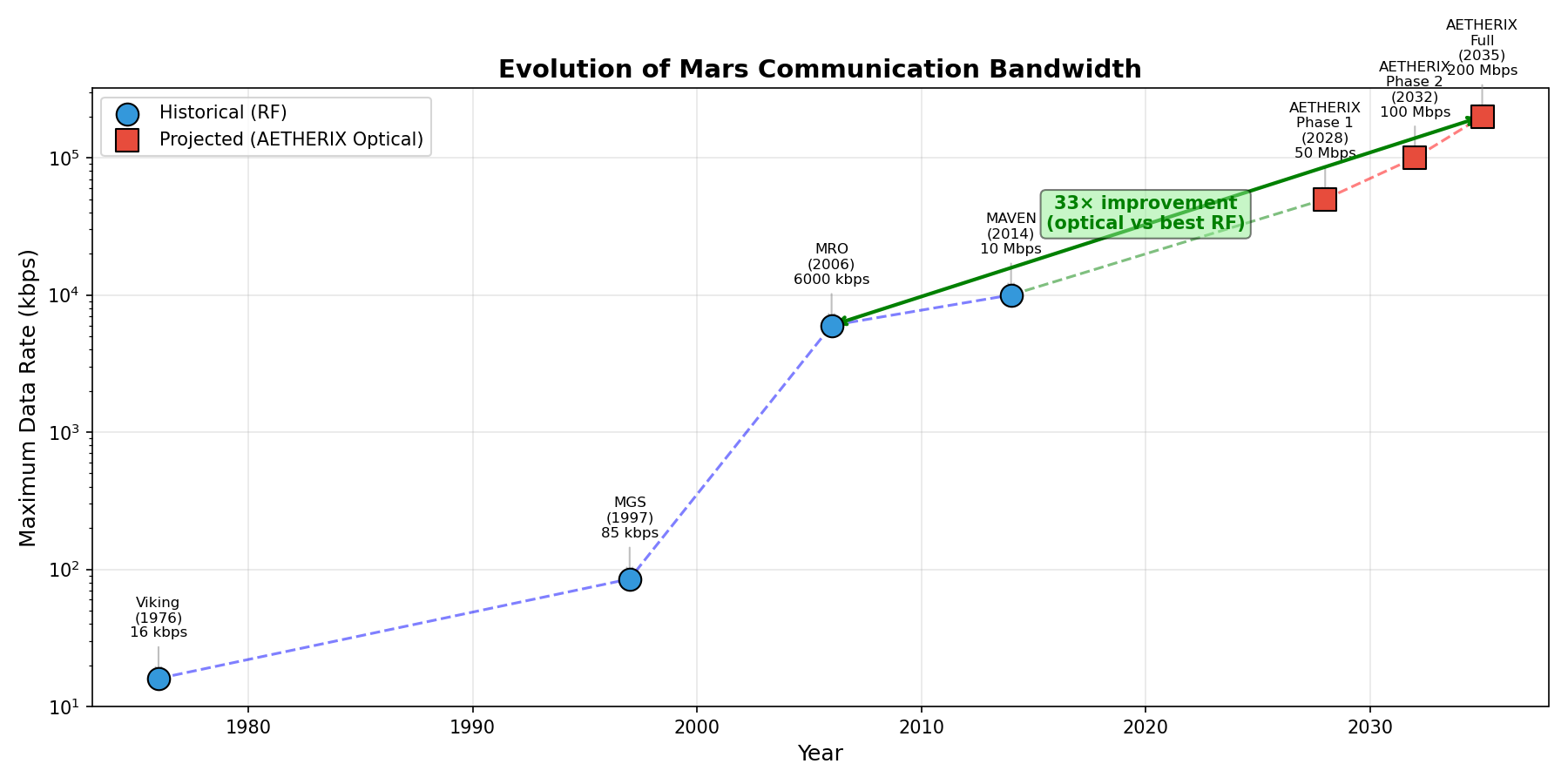
| Downlink Speed | 0.5–6 Mbps | 2–200 Mbps | 10–100× |
| Daily Data Volume | 5–10 GB | 50–100 GB | 10–20× |
| Availability | 60–75% | >95% | +20–35% |
| Routing | Static (CGR) | AI-Adaptive (RL) | Autonomous |
| Security | AES-256 | QKD + Post-Quantum | Future-proof |
| Scalability | 5–10 assets | 241 nodes | 10–100× |
| Solar Conjunction | Complete blackout | 50–70% via Lagrange relays | +50–70% |
Scientific Discovery
More data means more science. High-resolution imagery, spectral analysis, atmospheric measurements, and real-time telemetry from rovers, orbiters, and landers.
Human Missions
Reliable communication is critical for crewed Mars missions. Astronauts need to communicate with Mission Control, receive emergency updates, and transmit medical data.
Autonomous Operations
With AI routing, the network operates autonomously during blackouts and unexpected events — critical when you can’t wait 20+ minutes for a response from Earth.
Future-Proof Security
Quantum computers will eventually break current encryption. QKD provides information-theoretic security that no computer, classical or quantum, can ever break.
Phase 1: Earth → Lunar (2028–2030)
Deploy QKD between ground stations and lunar orbiters. Validate optical links at ≤400,000 km with 1.3s round-trip delay. Establish the first quantum-secured space link.
Phase 2: Earth → Mars Relay (2030–2035)
Deploy Lagrange-point relays and Mars orbiters. RL routing agents begin training on real contact windows. Target: 50 Mbps average, >90% availability.
Phase 3: Full Network (2035+)
Scale to 241 nodes across all 5 tiers. Federated RL agents across the full mesh. QKD key exchange via quantum repeaters. Target: 200 Mbps at closest approach, supporting human missions.
Microsoft’s AI disaster-assessment framework (satellite imagery → rapid damage maps). Adopted as AETHERIX’s payload layer: imagery triage that concretely generates EMERGENCY vs BULK bundles instead of abstract traffic.
MIT · Q4PyTorch geospatial ML library with pre-trained Sentinel-2/Landsat weights. Trains the triage models whose outputs become BPv7 priority classes — research-side only, never a core dependency.
MIT · Q4NASA Ames’ web-based mission-control framework, flown on real missions. The flight-ops console for ops-handbook drills — complementing Grafana’s platform/SRE view with a mission-ops view.
Apache-2.0 · Q4JPL’s flight-proven C++ framework (Ingenuity Mars Helicopter), with a CFDP stack. The flatsat “Mars asset” option — making F´-CFDP ↔ AETHERIX-BPv7 file delivery a first-class interop experiment.
Apache-2.0 · Q3docs/ROADMAP_12MO.md.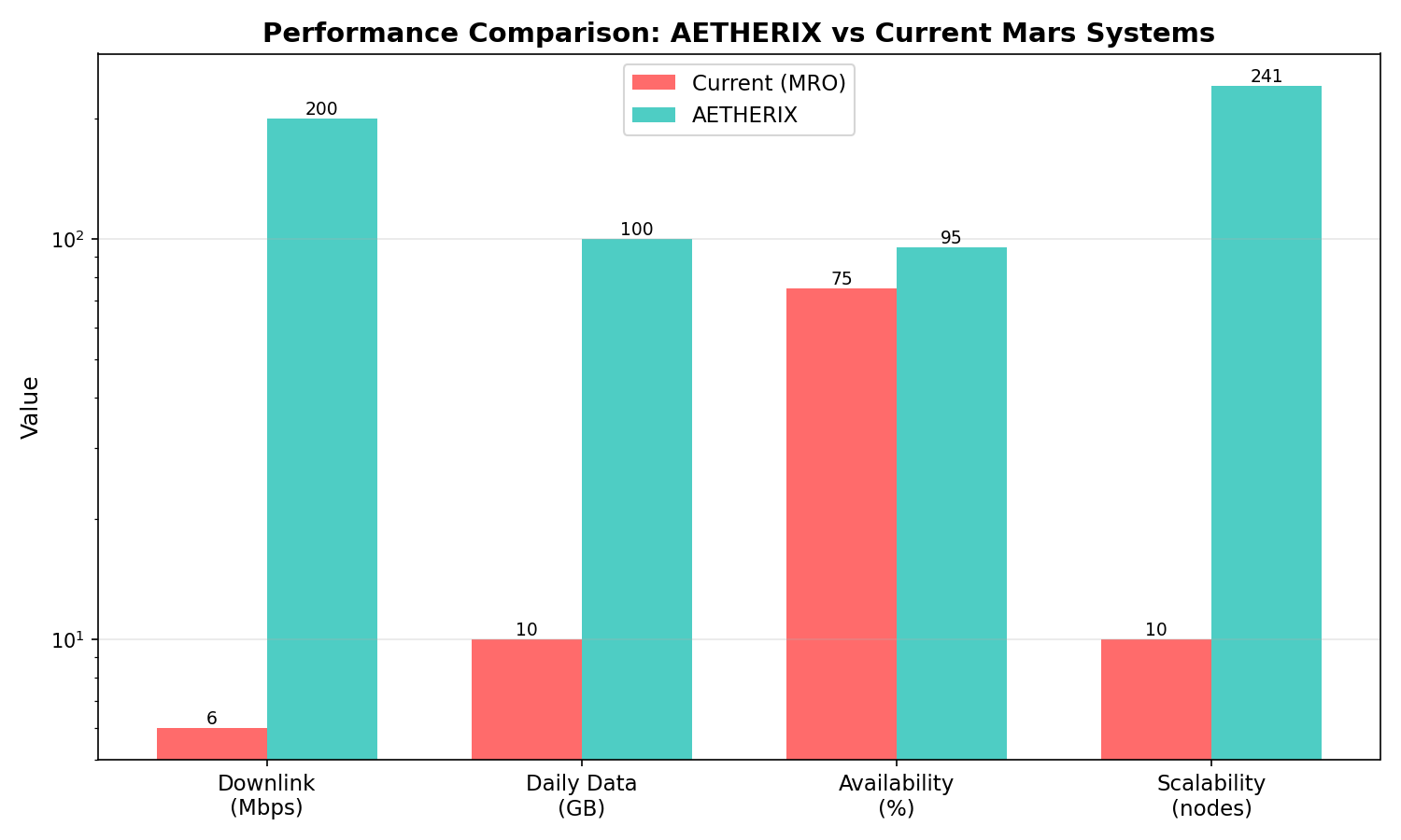
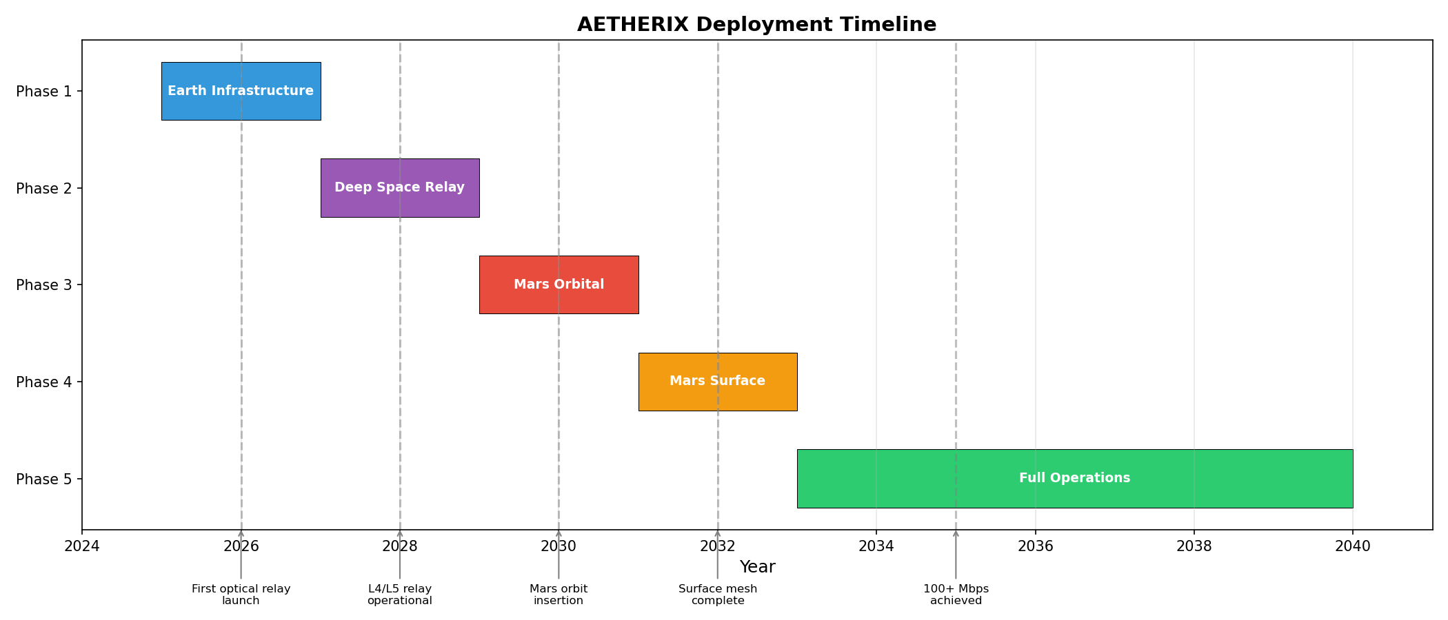
src/routing/dqn_agent.py, stdlib-only, trained under the deterministic safety shield) and the examiner’s distance test enshrined as CI (tests/test_distance_sensitivity.py: 55/225/401 M km runs must differ). Phases 5–8 target ns-3 integration, DQN productionisation, optical hardware demonstration, and decoy-state QKD validation — quarter-gated in docs/ROADMAP_12MO.md.Glossary
A complete reference of every technical term, acronym, and concept used across the AETHERIX platform — each with a plain-language definition, a worked example, and a citation.
The IETF standard (RFC 9171) that defines how data is packaged, addressed, and transported across networks with long delays and intermittent connections. The core protocol of DTN.
Example: A 500 MB rover scan becomes one bundle with a source, destination, priority and lifetime. It survives seven hops to Earth without any end-to-end connection ever existing.
A networking approach designed for environments where connections are intermittent, delays are extreme, and traditional protocols like TCP/IP fail. Think “postal service for data.”
Example: Posting a letter rather than making a phone call. The call needs both ends live at once; the letter is held at each post office until the next route opens.
A reliable transport protocol (RFC 5326) designed for links with very long round-trip times. Provides assured delivery over single hops in the DTN architecture.
Example: Used on the Earth–Mars deep-space hop. It splits data into a “red part” that is retransmitted until acknowledged and a “green part” that is not, so it never waits for a round trip to open a session.
A convergence layer (RFC 7242) that adapts BPv7 to use TCP for reliable delivery on the Earth segment, where low-delay, persistent connections are available.
Example: Used on the Earth-side segment between DSN sites and mission control, where a normal reliable TCP stream already exists and round trips are milliseconds.
A convergence layer that uses UDP for fast delivery over optical inter-satellite links. Trades guaranteed delivery for speed, with fragmentation and loss simulation.
Example: Used inside the 48-satellite LEO laser mesh, where latency is tiny and loss is bursty rather than congestive — so TCP’s congestion control would hurt more than help.
Consultative Committee for Space Data Systems. An international standards body that defines communication protocols for space missions. Used by NASA, ESA, JAXA, and others.
Example: The space-agency equivalent of the IETF. CCSDS 734.2-B-1 is the space profile of BPv7; CCSDS 141.0-B-1 covers the optical physical layer AETHERIX models.
The IETF standard that formally defines Bundle Protocol v7 — the core DTN data format, including primary blocks, extension blocks, and processing rules.
Example: The document that defines what a bundle actually is — primary block, payload block, lifetime, priority. AETHERIX’s bundle.py implements this structure directly.
The IETF standard that defines the Licklider Transmission Protocol (LTP) — designed for reliable data transmission over links with very long delays.
Example: Specifies LTP. The key idea is that the sender does not need an acknowledgement to keep transmitting — essential when an ACK takes 22 minutes to come back.
A static routing approach that pre-computes paths through a DTN using a graph of known future contacts. Deterministic but cannot adapt to unexpected changes.
Example: Plans a route from a published schedule: “Madrid sees Mars 16:00–24:00.” If the link fails at 17:00, CGR keeps following the stale plan — which is exactly the weakness AETHERIX’s RL agent addresses.
The CCSDS standardisation of Contact Graph Routing. It computes routes from a pre-published schedule of when links will exist, rather than from live network state. This is the static baseline AETHERIX’s reinforcement-learning agent replaces.
Example: A ground operator publishes a contact plan saying “Mars orbiter and DSN Madrid are in view 14:00–22:00 tomorrow.” SABR plans the whole route from that table in advance. If the link fails at 15:00, SABR keeps following the stale plan.
The security extension to BPv7. It adds integrity and confidentiality blocks to a bundle so that each hop can verify the payload has not been altered, without needing an end-to-end session.
Example: A bundle leaves Mars with an integrity block. Six hops later, a Lagrange relay can check the payload is unmodified on its own — it does not need to contact the sender, which would cost 44 minutes.
NASA’s reference implementation of the Bundle Protocol — the flight-proven DTN software actually used on spacecraft. It is the production system AETHERIX’s simulation is measured against.
Example: ION has flown on the International Space Station and on deep-space missions. AETHERIX does not use ION; it implements BPv7 independently so every component is inspectable, and cites ION as the interoperability target.
The software component on each node that actually does the BPv7 work: accepting bundles, taking custody, storing them, choosing a next hop, and forwarding when a contact opens.
Example: Every one of AETHERIX’s 241 nodes runs a BPA. When a rover generates science data, its BPA wraps it into a bundle and holds it until the orbiter comes overhead.
How long a bundle is allowed to remain in the network before it is discarded as stale. Set by the sender, it stops undeliverable data from filling buffers forever.
Example: An emergency alert might have a 2-hour lifetime — after that it is worthless. A bulk science file might have 30 days, because it is still useful whenever it arrives.
The acknowledgement one node sends back to the previous custodian to say “I have accepted responsibility for this bundle; you may now free your buffer.” Custody transfer is not complete until this arrives.
Example: A Mars orbiter forwards a bundle to an L4 relay and keeps its own copy. Only when L4’s custody signal comes back does the orbiter delete it — so a failure mid-transfer never loses the data.
The pre-computed schedule of which nodes will be able to talk to which, and when. Derived from orbital mechanics, it is the input Contact Graph Routing depends on.
Example: “Goldstone sees Mars 08:00–16:00; Madrid sees it 16:00–24:00.” That table is a contact plan. Its weakness is that it describes the future as predicted, not as it turns out.
The largest block of data a link can carry in one piece. Anything larger must be fragmented before transmission and reassembled afterwards.
Example: A 500 MB science bundle cannot cross a link with a 64 KB MTU in one go, so BPv7 fragments it — which is also how AETHERIX fills the tail of a closing contact window instead of leaving it idle.
Any endpoint in the DTN network — a satellite, rover, ground station, relay, or habitat. Each node can store, forward, and route bundles.
Example: AETHERIX has 241 of them, from DSN ground stations down to individual Mars surface sensors. Each one runs a Bundle Protocol Agent and can take custody.
The fundamental data unit in DTN. Like a network packet but smarter — it carries its own address, priority, lifetime, and custody tracking information. Designed to survive long delays.
Example: The DTN equivalent of a packet, but self-contained: it carries everything needed to be delivered later, including its own lifetime and priority, because no session exists to hold that state.
A responsibility handoff mechanism. When a node accepts custody of a bundle, it guarantees the bundle will not be lost — even if the original sender goes offline.
Example: A Mars orbiter forwards a bundle to an L4 relay but keeps its copy. Only when L4 signals “I have custody” does the orbiter delete it — so a mid-transfer failure never loses data.
The core DTN delivery model. Data is stored at each intermediate node until the next connection becomes available, then forwarded. No end-to-end connection required.
Example: In AETHERIX’s baseline run, 183 of 288 bundles are sitting in custody at intermediate nodes at the 24-hour mark. They are not lost — they are waiting for their next contact window.
A protocol adapter that sits between BPv7 and the physical link. Each transport type (TCP, UDP, LTP) has its own convergence layer, letting BPv7 work over any link technology.
Example: The adapter between BPv7 and whatever link is actually underneath. AETHERIX uses three: LTP for deep space, TCPCL for Earth, UDP-CL for optical inter-satellite links.
A scheduled period during which two nodes can communicate. Contact windows are predicted from orbital mechanics and define when data can be sent or received.
Example: “Optimal” windows run 8–12 hours at 99% availability; at solar conjunction the window drops to zero for two to four weeks.
The DTN addressing format. Looks like dtn://node/service. Identifies the source and destination of a bundle, similar to an IP address but designed for delay-tolerant operation.
Example: Written dtn://mars.surface.rover-01/science. Unlike an IP address it names a destination role, not a reachable host — which is what lets you address somewhere currently unreachable.
A measure of the power radiated by an antenna in a specific direction, combining transmitter power and antenna gain. Key metric in link budget calculations.
Example: AETHERIX’s 5 W, 22 cm optical terminal produces 144.4 dBm EIRP. It is the first term in the link-budget waterfall — how much power effectively heads toward the receiver.
A communication link between two satellites, typically using optical (laser) or RF technology. Enables data relay without passing through a ground station.
Example: The 10 Gbps optical links between AETHERIX’s 48 LEO satellites. Because there is no atmosphere between them, these are the fastest links in the whole architecture.
A standard pattern for arranging satellites in a constellation, defined by three numbers: total satellites, number of orbital planes, and the phase offset between planes. It gives even, predictable coverage.
Example: AETHERIX’s 48-satellite LEO laser mesh in Tier 2 is arranged this way. The pattern matters because it determines whether there is always a satellite overhead — and therefore whether a ground station ever goes dark.
Mission Operations Centre and Science Operations Centre. MOC flies the spacecraft — commanding, health, safety. SOC handles what the mission is for — planning observations and processing the science data.
Example: In AETHERIX’s Tier 1 these are two of the five ground nodes. A P0 emergency bundle is destined for the MOC; a 500 MB terrain scan is destined for the SOC.
The long-term vision DTN was invented to serve: a permanent, standards-based network spanning multiple planets, rather than a set of bespoke point-to-point links rebuilt for every mission.
Example: Today each Mars mission largely builds its own relay arrangements. An interplanetary internet means a new lander could join an existing network the way a new laptop joins Wi-Fi.
A graph algorithm that explores a network layer by layer, guaranteeing it finds the path with the fewest hops. AETHERIX uses it to generate candidate routes across the 241-node topology.
Example: BFS answers “what are the possible ways from this Mars rover to Earth?” The reinforcement-learning agent then decides which of those candidates to actually use, based on live link quality and buffer state.
The DSN ground stations on Earth: Goldstone (California), Madrid (Spain), and Canberra (Australia). These are the primary Earth-side endpoints for transmitting and receiving data.
GEO relay satellites and a constellation of 48 LEO satellites with laser crosslinks. Aggregates and routes data from ground stations toward deep space.
Relay stations at the Earth-Sun Lagrange points (ES-L4, ES-L5). Provide critical routing during solar conjunction when direct Earth–Mars links are blocked by the Sun.
Areostationary and polar-orbit relay satellites around Mars. Receive data from deep space and distribute it to surface assets, or collect surface data for return to Earth.
End-user assets on Mars: habitats, rovers, drones, sensor networks, and science instruments. The final destinations and sources of interplanetary data.
NASA’s global network of large radio antenna dishes at Goldstone (USA), Madrid (Spain), and Canberra (Australia). Provides continuous coverage for deep space communication.
Example: Goldstone, Madrid and Canberra, spaced roughly 120° apart in longitude so at least one always has line of sight to a target as Earth rotates.
An orbit at 35,786 km altitude where a satellite appears stationary relative to a point on Earth. Used for relay satellites that maintain constant position over ground stations.
Example: 35,786 km up, orbiting once per day so it appears fixed overhead. AETHERIX puts three GEO relays in Tier 2 as the bridge between the LEO mesh and deep space.
An orbit below 2,000 km altitude. AETHERIX uses a constellation of 48 LEO satellites with optical crosslinks to form a laser mesh network around Earth.
Example: Where AETHERIX’s 48-satellite laser mesh sits. Low altitude means short hops and high rates, but any single satellite is only overhead for minutes at a time.
A gravitationally stable position in a two-body orbital system where a smaller object can maintain a fixed position. AETHERIX uses Earth-Sun L4 and L5 for relay stations.
Example: ES-L4 and ES-L5 sit 60° ahead of and behind Earth in its orbit. That geometry keeps a line of sight to Mars around the solar limb when the direct path is blocked by the corona.
The loss of signal strength that occurs as a signal spreads out while traveling through free space. Increases with the square of the distance — a major challenge for interplanetary links.
Example: At Mars opposition it is about −353 dB, and at conjunction about −370 dB. Computed from 20·log₁₀(4πd/λ) — a single number that explains why deep space is hard.
A complete accounting of all gains and losses in a communication link, from transmitter output to receiver input. Determines whether a link can close — i.e., deliver enough signal to be usable.
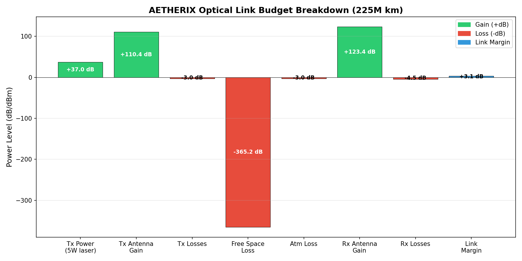
Example: Add every gain, subtract every loss, and see whether anything usable arrives. AETHERIX’s optical budget closes at +4.31 dB at opposition; Ka-band at the same rate does not close at all.
The difference between the received signal power and the minimum power required for reliable communication. Positive margin means the link works; more margin means more reliability.
Example: Positive means the link works. AETHERIX reports +4.31 / +3.33 / +3.08 dB at 55M / 225M / 401M km — and those are uncoded, so they are a floor rather than a prediction.
The ratio of desired signal power to background noise power. Higher SNR means clearer, more reliable communication. Measured in decibels (dB).
Example: AETHERIX requires 10 dB of SNR for its target bit error rate. Below that, the receiver cannot reliably tell a real photon from detector noise.
The diameter of a telescope or antenna. Larger apertures collect more signal and produce narrower beams, enabling longer-range communication.
Example: Bigger collects more light and produces a tighter beam. AETHERIX models a 22 cm flight aperture against a 5 m ground telescope — the same asymmetry DSOC flies.
A near-infrared wavelength used for space optical communications. Chosen for its eye safety, low atmospheric absorption, and compatibility with terrestrial fiber-optic components.
Example: Chosen because the entire terrestrial telecom industry already builds lasers, amplifiers and detectors at this wavelength. NASA’s DSOC flies at exactly 1550 nm too.
26.5 GHz. High data rate but weather-sensitive. Primary RF band for high-throughput Mars downlink.
8.4 GHz. Moderate data rate with good all-weather performance. Used by most current Mars missions.
2.3 GHz. Lower data rate but highly reliable. Used for command uplink and emergency communications.
401 MHz. Ultra High Frequency. Short range, used for surface-to-orbiter links on Mars.
The change in frequency of a signal caused by relative motion between transmitter and receiver. Must be compensated for in space links.
Example: At 24 km/s relative velocity, a Ka-band carrier shifts by ±2.1 MHz. Without pre-compensation the receiver never acquires lock — the signal is outside the loop bandwidth.
Signal loss from Earth’s atmosphere — clouds, rain, and gases absorb RF and optical signals. Optical links are more affected than RF. Typically 1–5 dB loss depending on weather.
Example: AETHERIX budgets −3 dB for clear sky. Cloud makes an optical link fail entirely, which is precisely why Ka-band RF is kept as the always-available fallback.
Signal loss from imperfect antenna/telescope alignment. Optical beams diverge only ≈5 μrad, so even tiny misalignments cause significant loss. Typically 1–3 dB per endpoint.
Example: AETHERIX budgets −1.0 dB at the transmitter and −0.5 dB at the receiver. At 494 million km you must aim at where Earth will be when the photons arrive, not where it is.
NASA’s technology demonstration that proved laser communications work at interplanetary distance. It flies aboard the Psyche spacecraft, launched 5 October 2023, and is the flight heritage behind AETHERIX’s optical design.
Example: On 11 December 2023 DSOC sent ultra-high-definition video from 31 million km at 267 Mbps. On 3 December 2024 it downlinked from 494 million km — further than Earth and Mars ever get apart.
A way of encoding data in when a light pulse arrives rather than how bright it is. Time is divided into slots, and which slot contains the photon carries the information.
Example: With 16 slots, a single detected photon carries 4 bits. That photon efficiency is why deep-space optical uses PPM — at Mars range you may receive fewer photons than you sent bits.
PPM combined with a powerful forward-error-correction code. The coding lets the receiver recover the data correctly even when a large fraction of photons are lost or arrive in the wrong slot.
Example: SCPPM is what DSOC actually flies. It is worth roughly 13 dB — and because AETHERIX’s link budget deliberately excludes it, AETHERIX’s reported margins are a conservative floor.
How much weaker a signal can be, in decibels, and still be decoded correctly once forward-error correction is applied. It is the difference between what raw physics allows and what a real coded system achieves.
Example: AETHERIX’s uncoded budget returns −12.8 dB at DSOC’s demonstrated operating point. Since DSOC closed that link, roughly 13 dB of coding gain is exactly what the model leaves out.
A photon detector cooled to a few kelvin. A single arriving photon deposits enough energy to break superconductivity in the nanowire, producing a measurable voltage pulse — so individual photons can be counted.
Example: DSOC’s downlink receiver at Palomar Observatory is exactly this. The same detector family is used in QKD receivers, because both problems are “count single photons reliably.”
How quickly a transmitted beam spreads out with distance, set by wavelength divided by aperture. Narrower divergence means more of the transmitted energy lands on the receiver instead of missing it.
Example: A 1550 nm laser has a wavelength about 10,000× shorter than Ka-band radio, so for the same telescope size the beam is far tighter. That single fact is the entire case for optical over RF.
The Earth-side half of an optical link. NASA’s Optical Communication Telescope Laboratory at JPL’s Table Mountain Facility transmits the uplink laser, which the spacecraft also uses as a pointing beacon.
Example: The uplink does double duty: it carries low-rate commands, and it gives the spacecraft something to lock onto so it knows precisely where to aim its own downlink beam.
A detector click that was not caused by a real photon — thermal noise in the detector itself. Dark counts set the noise floor of a photon-counting receiver and directly limit how far a link can reach.
Example: In QKD, dark counts show up as errors in the sifted key, raising QBER even with no eavesdropper present. That is part of why a real channel never reads 0% QBER.
How many bits are carried per detected photon. Conventional radio thinks in watts; deep-space optical thinks in photons, because at these distances photons arrive one at a time.
Example: High-order PPM can carry several bits per photon. This is why quoting an optical link in raw power alone is misleading — the modulation choice changes the achievable rate for the same received energy.
An AI technique where an agent learns optimal behavior through trial and error, receiving rewards for good decisions and penalties for bad ones.
Example: Learning to navigate a new city without a map: try streets, notice which get you there faster, and gradually stop trying the dead ends.
A value-based RL algorithm that learns a “quality” score (Q-value) for every possible action in every possible state. The agent picks the action with the highest Q-value.
Example: The agent stores a value for every (situation, action) pair and updates it with the Bellman equation after each outcome. After 800 episodes AETHERIX’s agent converges on forwarding in 713 of 800 decisions.
A lookup table that maps every network state to a value for each possible routing action. The agent’s “cheat sheet” built from experience. For larger networks, replaced by neural networks (DQN).
Example: A literal lookup table you can print and inspect row by row. That auditability is why AETHERIX uses one instead of a neural network — every routing decision can be explained.
A policy that mostly chooses the best-known action (exploitation) but occasionally tries a random one (exploration) with probability epsilon. Balances known good paths vs. discovering better ones.
Example: AETHERIX starts at ε = 1.0 (fully random) and decays by 0.995 per episode, reaching 0.018 after 800 episodes — about 98% exploiting what it has learned.
A multi-objective scoring formula: R = α(delivery) − β(delay) − γ(hops) − δ(drops) − ε(energy). Guides the RL agent toward reliable, fast, efficient routing.
Example: R = +1.0(delivery) − 0.001(delay) − 0.1(hops) − 10.0(drops) − 0.01(energy). The drop penalty is ten times the delivery reward, which makes discarding a bundle strictly irrational.
A distributed machine learning approach where multiple nodes train locally and share only model updates (not raw data). Enables collaborative learning across the DTN.
Example: Each of the 241 nodes trains on what it can see locally, then they periodically merge Q-tables. Knowledge is shared without shipping raw telemetry across an expensive link.
A neural network that approximates the Q-table, enabling RL to scale to large state spaces. The production upgrade path from the current Q-table approach in AETHERIX.
Example: A neural network replacing the Q-table, which generalises to situations never seen before. AETHERIX deliberately does not use one — it is roadmap Phase 6, traded away for auditability.
The fundamental trade-off in reinforcement learning. Exploiting means taking the best action you currently know; exploring means trying something else in case it turns out better.
Example: Always exploiting means never discovering a better route. Always exploring means never using what you learned. AETHERIX resolves it with ε-greedy: explore often at first, then decay to almost pure exploitation.
Deliberately choosing the weights in a reward function so the agent learns the behaviour you actually want, rather than something that merely scores well.
Example: AETHERIX sets the drop penalty to 10.0 against a delivery reward of 1.0. That asymmetry makes discarding a bundle strictly irrational — the agent stores and waits instead. Late beats lost for science data.
A running average that weights recent samples more heavily than old ones, so it tracks change quickly without storing history.
Example: AETHERIX uses it to track link quality. A link that just degraded should influence the routing decision more than how it behaved an hour ago — and EWMA does that in one number per link.
A method of creating shared secret keys using quantum physics. Any eavesdropping attempt disturbs the quantum states and is immediately detectable.
The Bennett-Brassard 1984 QKD protocol. Uses polarized photons in two bases to establish a shared key. If an eavesdropper intercepts, the error rate rises above 11%.
The Ekert 1991 QKD protocol. Uses entangled photon pairs and Bell inequality tests to establish a key and detect eavesdropping simultaneously.
The error rate in quantum key transmission. If QBER is below 11%, no eavesdropper is present and the key is secure. Above 11%, the key is discarded.
Example: AETHERIX measures 0.0% on a clean channel and 24.7% under intercept-and-resend. It is a security parameter that bounds leakage — not an on/off eavesdropper alarm.
The basic unit of quantum information. Unlike a classical bit (0 or 1), a qubit can be in a superposition of both states simultaneously. Measuring collapses it.
Example: In BB84 each qubit is a single photon’s polarisation. Unlike a classical bit it has no definite value until measured, and measuring it in the wrong basis destroys the original state.
A device that extends QKD range through entanglement swapping. Links short-distance quantum segments into a long-distance quantum channel.
Example: Needed because direct QKD key rate falls as 1/d² — at Mars range that is effectively zero bits per second. Chaining entanglement swaps through Lagrange relays is what makes the link possible.
Cryptographic algorithms designed to resist attacks by quantum computers. Relies on mathematical problems hard for both classical and quantum computers.
Example: Classical algorithms chosen to resist a quantum attacker. AETHERIX pairs them with QKD because QKD distributes keys but cannot authenticate — you need both.
A NIST-standardized post-quantum key encapsulation mechanism. Used for securely exchanging encryption keys in a way that resists quantum computer attacks.
Example: Standardised by NIST as ML-KEM in FIPS 203 (2024). If you see both names, they are the same algorithm — Kyber was the submission, ML-KEM is the standard.
A NIST-standardized post-quantum digital signature scheme. Used for authenticating messages and verifying identity in a quantum-resistant way.
Example: Standardised by NIST as ML-DSA in FIPS 204 (2024). This is the signature half, and it is what stops a man-in-the-middle attack on the QKD reconciliation channel.
A technique that reduces any partial information an eavesdropper might have about a key, by distilling a shorter, completely secret key from a longer one.
Example: Take 600 partially-compromised bits, run them through a universal hash, keep 400. You do not work out which bits leaked — compression destroys the eavesdropper’s partial knowledge wholesale.
A fundamental law of quantum physics: it is impossible to create an identical copy of an unknown quantum state. This is why QKD is secure — eavesdroppers cannot copy qubits.
Example: Wootters & Zurek, 1982. It is why an eavesdropper cannot simply copy a photon and forward the original — the universe forbids it, so she must measure and thereby disturb.
A quantum phenomenon where two particles share correlated states, regardless of distance. Measuring one instantly determines the other. Einstein called it “spooky action at a distance.”
Example: Two photons whose measurement outcomes stay correlated no matter how far apart they are. E91 uses this instead of prepare-and-measure, and it is what entanglement swapping chains together.
The step after transmission where Alice and Bob publicly compare which basis they each used for every photon — never the bit values — and keep only the bits where the bases matched. Roughly half survive.
Example: Send 1,000 photons, keep about 500. That one-half is the q in the key-rate formula. Announcing a basis leaks nothing: knowing Alice asked the Z question says nothing about whether her answer was 0 or 1.
Correcting the remaining differences between Alice’s and Bob’s sifted keys over a public channel, so both end up with an identical string. Necessary because a key that differs by even one bit is useless.
Example: They exchange parities of blocks and binary-search to the mismatched bit. Everything said is public, so this step leaks information — which privacy amplification then has to remove.
The standard information-reconciliation protocol for QKD. It runs several passes of block-parity comparison with shuffled block boundaries, binary-searching down to each error.
Example: Implemented in privacy_amplification.py. Its cost is measured in leaked bits: roughly h₂(Q)×n bits of information about an n-bit key become public.
A measure of uncertainty in a two-outcome random variable: h₂(Q) = −Q·log₂Q − (1−Q)·log₂(1−Q). In QKD it converts an error rate into an amount of leaked information.
Example: The surviving fraction of a sifted key is 1 − 2·h₂(Q). Binary entropy reaches ½ at Q ≈ 0.11 — which is exactly why 11% is the abort threshold: the formula returns zero bits there.
A defence against attacks that exploit multi-photon pulses. The transmitter randomly varies pulse intensity, and the yields are compared per intensity — an attack affects them differently, so it becomes visible.
Example: AETHERIX does not implement decoy states; its model assumes a true single-photon source. This is a known limitation, scoped as roadmap Phase 8.
The attack decoy states defend against. Real transmitters use attenuated laser pulses that sometimes contain more than one photon; an eavesdropper keeps one and forwards the rest.
Example: Critically, PNS leaks key material without raising QBER at all — so QBER-based detection cannot see it. This is why an ideal-single-photon model is optimistic for real hardware.
A statistical test that distinguishes genuine quantum entanglement from any classical explanation. If measured correlations exceed the classical bound (S > 2), the particles really were entangled.
Example: E91 uses this instead of the no-cloning theorem: if the Bell inequality is violated, no eavesdropper could have been present, because measuring would have destroyed the correlation.
The mechanism that makes quantum repeaters possible. Two separately entangled pairs are joined by a measurement in the middle, leaving the two outer particles entangled despite never having interacted.
Example: Direct QKD to Mars is impossible — key rate falls as 1/d², reaching effectively zero. Chaining entanglement swaps through Lagrange relays is how the interplanetary segment becomes feasible at all.
The NIST-standardised post-quantum key encapsulation mechanism, derived from CRYSTALS-Kyber. It establishes a shared secret using maths believed hard even for a quantum computer.
Example: AETHERIX pairs this with QKD: QKD distributes keys with physics-based security, ML-KEM provides a classical fallback wherever a quantum channel is unavailable.
The NIST-standardised post-quantum digital signature algorithm, derived from CRYSTALS-Dilithium. It provides authentication that survives a quantum adversary.
Example: This matters because QKD distributes keys but does not authenticate. Without a signature layer, QKD is open to a man-in-the-middle. ML-DSA fills exactly that gap.
Security accounting for the fact that real sessions exchange a finite number of photons. Asymptotic formulas assume infinitely many, so they overstate the extractable key for short sessions.
Example: AETHERIX’s bound R ≈ q[1 − 2h₂(Q)] is asymptotic. A real deployment must subtract a statistical-fluctuation term — scoped as roadmap Phase 8.
The threat model that justifies deploying quantum-resistant security today. An adversary records encrypted traffic now and stores it, waiting for a future quantum computer to break it.
Example: A Mars architecture designed now will still be operating in 20–30 years. Traffic intercepted today is still sensitive then — so computational security alone is not sufficient.
The 2000 security proof for BB84 that established the 11% QBER threshold, by showing BB84 is equivalent to an entanglement-purification protocol whose security can be proven directly.
Example: This is the citation behind “QBER < 11%”. It is a statement about how much key can be extracted, not a detector that flags an eavesdropper.
The 1978 information-theory result underpinning QKD: a secret key can be distilled whenever Alice and Bob share more mutual information with each other than either shares with an eavesdropper.
Example: It is the reason privacy amplification works at all — it says how much key can be salvaged from a partially compromised string, given the measured QBER.
The classical encryption workhorses. AES-256 is symmetric (same key both ends); RSA is asymmetric and used for key exchange. Both rest on computational hardness, not physical law.
Example: RSA is the one that breaks first under a quantum computer running Shor’s algorithm. AES-256 is weakened but not broken. QKD replaces the key-exchange step precisely because that is the vulnerable half.
A cryptographic hash function producing a fixed 256-bit fingerprint of any input. Any change to the input, however small, produces a completely different output.
Example: AETHERIX uses it in bundle integrity: each bundle is hashed and signed, so any relay can detect a single flipped byte without contacting the sender.
The 780-day cycle over which Earth and Mars repeat their relative positions. Distance goes from closest approach (opposition) to farthest (conjunction) and back.
The point of closest Earth–Mars distance, approximately 55 million km. Signal delay is at its minimum (~3 minutes one-way). Best conditions for communication.
The point of maximum Earth–Mars distance, approximately 401 million km, with Mars behind the Sun. Signal delay peaks at ~22 minutes one-way.
A ~2-week period around conjunction when the Sun lies directly between Earth and Mars, making direct communication impossible. Mitigated via Lagrange relays.
The angular position of a planet in its orbit, measured from perihelion. Used to calculate real-time Earth–Mars distance and contact windows.
Example: The angle from perihelion to the body’s current position. It is the slider in AETHERIX’s orbital demo — drag it and watch Earth–Mars distance sweep from 54.6M to 401M km.
The closest point to the Sun in a planet’s orbit. Mars at perihelion is about 207 million km from the Sun.
Example: Mars at perihelion combined with Earth at the right point gives the 54.6 million km closest approach — the best case for any Mars communications link.
The farthest point from the Sun in a planet’s orbit. Mars at aphelion is about 249 million km from the Sun.
Example: Contributes to the 401 million km worst case. Between perihelion and aphelion the distance varies by a factor of 7.3, and data rate by far more, since it falls with distance squared.
The Mars equivalent of Earth’s geostationary orbit, at ~17,032 km altitude. A satellite here appears stationary over a fixed point on Mars.
Example: The Mars equivalent of geostationary, at 17,032 km altitude. A satellite there hovers over one spot on Mars, giving a surface base a permanently available relay.
149.6 million kilometers — the average distance from Earth to the Sun. Used as a standard unit for interplanetary distances. Mars orbits at ~1.52 AU.
Example: About 149.6 million km — the Earth–Sun distance. Mars sits at a semi-major axis of 1.524 AU, which is why its distance from Earth varies so dramatically.
The time it takes for a signal traveling at the speed of light to traverse the distance between two points. Earth–Mars: 3 to 22 minutes one-way.
Example: 3.1 minutes at opposition, 22.3 minutes at conjunction, one way. Double it for a round trip: 6 to 44 minutes. This single fact is why TCP cannot work and DTN must.
The orbital configuration where the Sun–Earth–Mars angle is about 90° — roughly halfway between opposition and conjunction, at intermediate distance.
Example: In AETHERIX’s orbital demo, quadrature sits at about 270 million km with roughly 15 minutes of one-way light time — between opposition’s 3 minutes and conjunction’s 22.
The NASA orbiter that has served as the primary Mars relay since 2006. Its published performance is the industry baseline AETHERIX measures itself against.
Example: MRO’s Ka-band return link runs at 0.5–6 Mbps with 60–75% availability. Every AETHERIX comparison cites this as the baseline — and labels it as NASA’s figure, not a measurement of its own.
Megabits per second. A unit of data transfer speed. AETHERIX achieves 2–200 Mbps depending on Earth–Mars distance.
Example: MRO’s published Ka-band return link is 0.5–6 Mbps. AETHERIX targets 2–200 Mbps — a capability derived from the link budget, and labelled a target rather than a measurement.
Decibels relative to 1 milliwatt. A unit of absolute power level. 0 dBm = 1 mW.
Example: Decibels relative to one milliwatt. AETHERIX’s 5 W laser is 36.99 dBm; the signal arriving at Earth is around −90 dBm — roughly a billionth of a billionth of a watt.
Decibels. A logarithmic ratio unit used to express gain or loss. +3 dB means double the power; −3 dB means half.
Example: A logarithmic ratio, so numbers add instead of multiplying. +3 dB is double the power, −3 dB is half. It is what makes a link budget a column of additions.
Total data successfully delivered per unit time. Distinct from bandwidth — throughput accounts for protocol overhead and losses.
Example: Distinct from link rate: it is what actually gets delivered end to end. AETHERIX’s 500 MB Mars-to-JPL journey takes ~13 minutes against a 12.5-minute light-time floor — under 5% overhead.
The end-to-end time from when data is sent to when it arrives. In interplanetary DTN, this includes propagation delay, storage time, and processing at each hop.
Example: In deep space this is dominated by physics, not equipment. No protocol improvement can beat the 3–22 minute light-time floor, which is why DTN optimises for delivery, not latency.
The percentage of time that communication is possible. Current Mars missions achieve 60–75%; AETHERIX targets >95% via multi-path routing and Lagrange relays.
Example: MRO’s published figure is 60–75%. AETHERIX targets >95% using Lagrange relays for conjunction coverage — and that figure is labelled a design target, not a measurement.
The fraction of bits received incorrectly. Deep-space links typically achieve 10−6 to 10−9 BER. Forward error correction (FEC) codes improve this by adding redundant bits for self-correction.
Example: AETHERIX designs to a 10⁻⁶ BER, which needs about 10 dB of SNR. One wrong bit in a million is tolerable for imagery; for a command sequence it is not, hence error correction.
A single charged particle flips one bit in memory or a register. The most common soft error in space; corrected by ECC.
Example: A cosmic ray flips one bit in memory. AETHERIX’s radiation module measures 37,159 raw upsets over a 210-day cruise on 512 Mbit of unprotected memory.
One energetic ion flips two or more adjacent bits at once. SECDED cannot correct it — defeated by physically interleaving the bits of a word.
Example: One particle strike corrupts several adjacent cells at once, which defeats codes that can only fix one bit per word. The fix is bit interleaving, so adjacent physical cells belong to different words.
A particle triggers a parasitic short that can destroy the chip unless power is cycled. Mitigated with current limiting and latchup-immune (rad-hard) parts.
Example: A strike triggers a parasitic structure that draws destructive current. Unlike a bit flip this can physically destroy the part, so mitigation is current limiting plus a power cycle.
Cumulative radiation dose (measured in krad) that slowly degrades electronics. The RAD750 tolerates ~200 krad — far above a Mars-mission dose.
Example: Cumulative damage rather than a single event — the part slowly degrades until it fails. The RAD750 gives roughly 2,127× margin over a 687-day Mars surface mission.
Three identical units compute in parallel; a voter outputs the majority, masking any single faulty unit. Fails only if two agree wrongly (≈3p² vs p).
Example: Run three copies of the same computation and take the majority vote. If one is corrupted, the other two outvote it. AETHERIX measures a 3,334× reliability gain from TMR alone.
Single Error Correct, Double Error Detect. A Hamming-code memory (e.g. 39,32) that fixes one flipped bit per word and flags two. ~22% storage overhead.
Example: Single Error Correction, Double Error Detection — a (39,32) Hamming code. It repairs one flipped bit per word and notices two, but cannot fix two, which is why scrubbing matters.
A background process that periodically re-reads and rewrites memory, repairing single-bit errors before a second upset accumulates and becomes uncorrectable.
Example: Periodically walk memory and repair single-bit errors before a second strike hits the same word. Without it, a correctable error eventually becomes an uncorrectable one.
Fault Detection, Isolation & Recovery. The autonomous logic that spots an anomaly, isolates the faulty unit, attempts recovery, and falls back to SAFE-MODE if it cannot.
Example: Fault Detection, Isolation and Recovery. Detect the fault, isolate the failing unit, reload it — and if the recovery budget runs out, drop to SAFE-MODE rather than fail silently.
A hardware timer that healthy software must periodically “kick.” If it expires (a hung CPU), it forces a reset — a last line of defense against radiation-induced lock-ups.
Example: A countdown the software must keep resetting. If it ever reaches zero, the system assumes the software has hung and reboots it. AETHERIX’s reaches SAFE_MODE after six ticks.
BAE Systems’ radiation-hardened flight processor used on Curiosity and Perseverance. ~200 krad tolerance, latchup-immune. ESA’s equivalent is the LEON3FT / GR712RC.
Example: The radiation-hardened PowerPC flown on Curiosity and Perseverance. Roughly 200 MHz — slower than a phone from 2005, but it survives an environment that would destroy the phone in days.
Treating traffic differently by importance. AETHERIX maps every bundle to one of four priority tiers so urgent data is always sent first.
Example: Deciding what moves first when the link cannot carry everything. AETHERIX uses five classes, and P0 emergency traffic preempts whatever is currently in flight.
P0 Emergency/Safety, P1 Mission-critical, P2 High-priority, P4 Low/Bulk — mapped onto BPv7 bundle priority for scheduling and preemption.
Example: P0 emergency (crew health, collision), P1 urgent (nav corrections), P2 normal (telemetry, science), P3 low (software updates), P4 bulk (archival). Five classes, strictly ordered.
An emergency bundle interrupts an in-progress lower-priority transfer, is sent immediately (often via a low-rate direct-to-Earth backup), then normal traffic resumes.
Example: A P0 emergency arrives while a bulk file is transmitting. Preemption stops the bulk transfer mid-flight and sends the emergency instead — the bulk data resumes afterwards.
Ordering transmissions by priority and then by earliest deadline; data that cannot arrive in time this contact is deferred rather than wasting the link.
Example: Within one priority class, send whatever expires soonest first. Combined with strict priority across classes, this is what stops a time-critical bundle ageing out in a buffer.
Shrinks data with no information loss (telemetry via CCSDS 121.0-B-3, Rice coding ≈ 3×). Used where every bit matters.
Example: Rice coding under CCSDS 121.0-B-3 gives roughly 3× on telemetry. Every bit is recoverable, which matters when the data is a command log rather than a picture.
Discards perceptually-minor detail for much higher ratios (imagery via CCSDS 122.0-B-2, wavelet ≈ 10×; video ≈ 50×). Used for bulk imagery.
Example: Wavelet compression under CCSDS 122.0-B-2 gives roughly 10× on imagery by discarding detail the eye will not miss. Acceptable for a landscape photo, not for a checksum.
Splitting a large BPv7 bundle so the portion that fits the current contact is sent and the remainder is deferred — keeping the link at full utilization.
Example: A contact window has four minutes left and the next bundle needs six. Fragmentation sends what fits and defers the rest, so the link is never left idle waiting for a whole bundle.
A minimal-power, beacon-only spacecraft state entered after repeated failures, preserving the vehicle while it waits for ground intervention.
Example: The spacecraft shuts down non-essential systems, points its antenna at Earth and waits for instructions. Deliberately boring — it is the state you want when nobody can reach you for 22 minutes.
Live Demo Walkthrough
Every command, the exact output to expect, what each number means, and the question most likely to follow. Verified against a live run on 2 September 2026 — Python 3.14.6, seed 42.
python run_simulation.py and talk over it. Six modules, no arguments, no external dependencies, deterministic on seed 42 — store-and-forward, link budget, RL convergence, conjunction recovery, QKD, and radiation hardening in a single command.Work down this list. If something misbehaves, drop a tier and say so plainly: “Rather than debug that in front of you, let me show you the same result from the simulation.”
| Tier | What | Why it is safe |
|---|---|---|
| 1 | python run_simulation.py | No network, no browser, no backend. Pure Python, zero external dependencies. |
| 2 | Showcase from localhost:8080 | Static HTML/JS. No backend, no network dependency. |
| 3 | ./scripts/run_demos.sh 1-6 | Six standalone CLI demos, each runs independently. |
| 4 | Read the source on GitHub | Always works. Content, not theatre. |
| ✗ | React app + FastAPI backend | Most moving parts. Two processes and a database — start before the call or not at all. |
The spine of the demo. One command, six modules, every learning outcome.
Baseline DTN store-and-forward
Hybrid link budget — optical vs Ka-band
LO-c · LO-dRL routing convergence
LO-gSolar-conjunction failure & recovery
Lead with this if short on timeIf asked why all rewards are negative: “The reward function charges for delay, hops and energy on every path — there is no free route. What matters is the ordering: −0.201 beats −1.438.”
BB84 quantum key distribution
LO-bRadiation-hardened computing
LO-eServe locally — cd docs && python3 -m http.server 8080 — and never depend on the network. All 15 demo tabs and 26 interactive controls were swept and verified working on 2 September 2026.
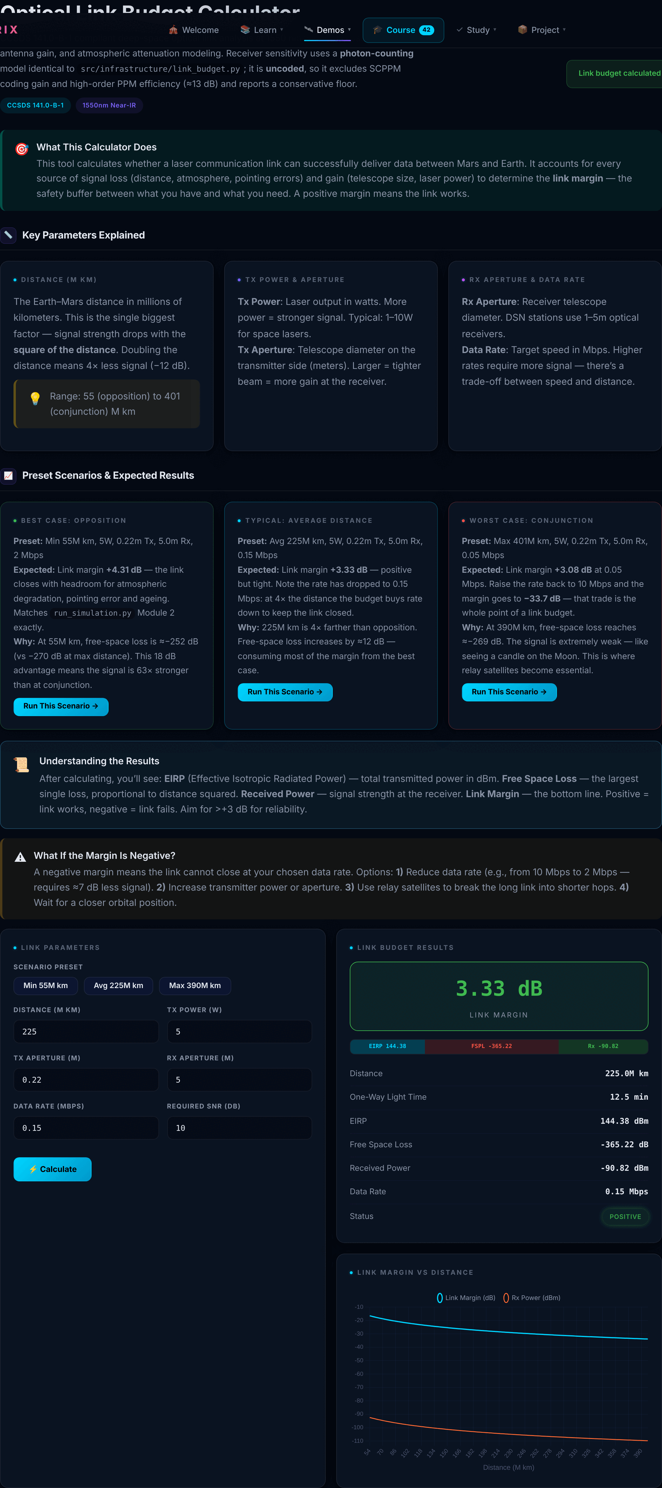
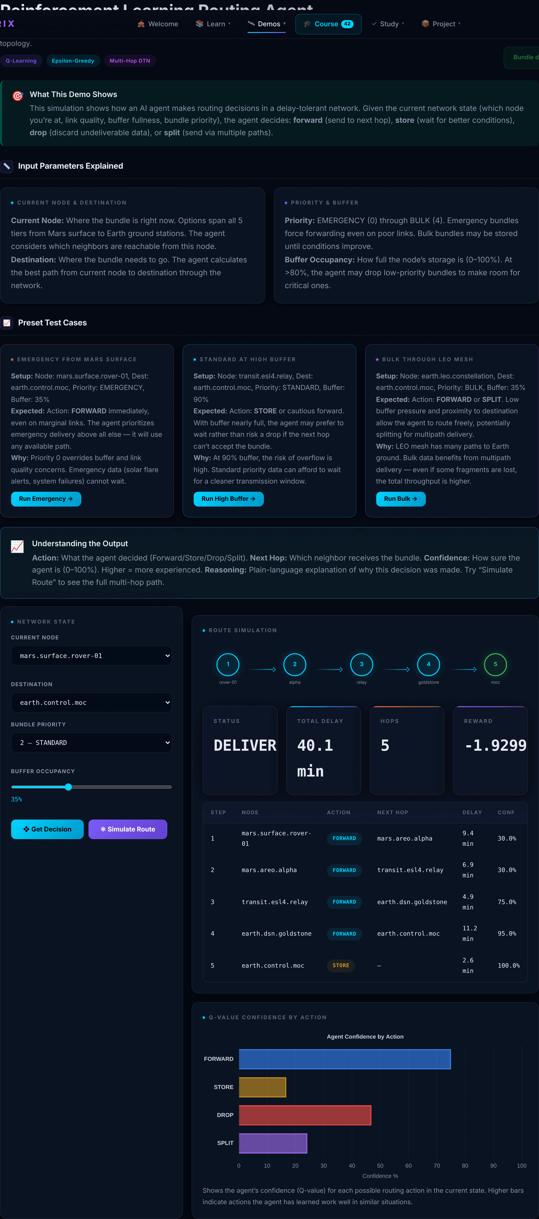
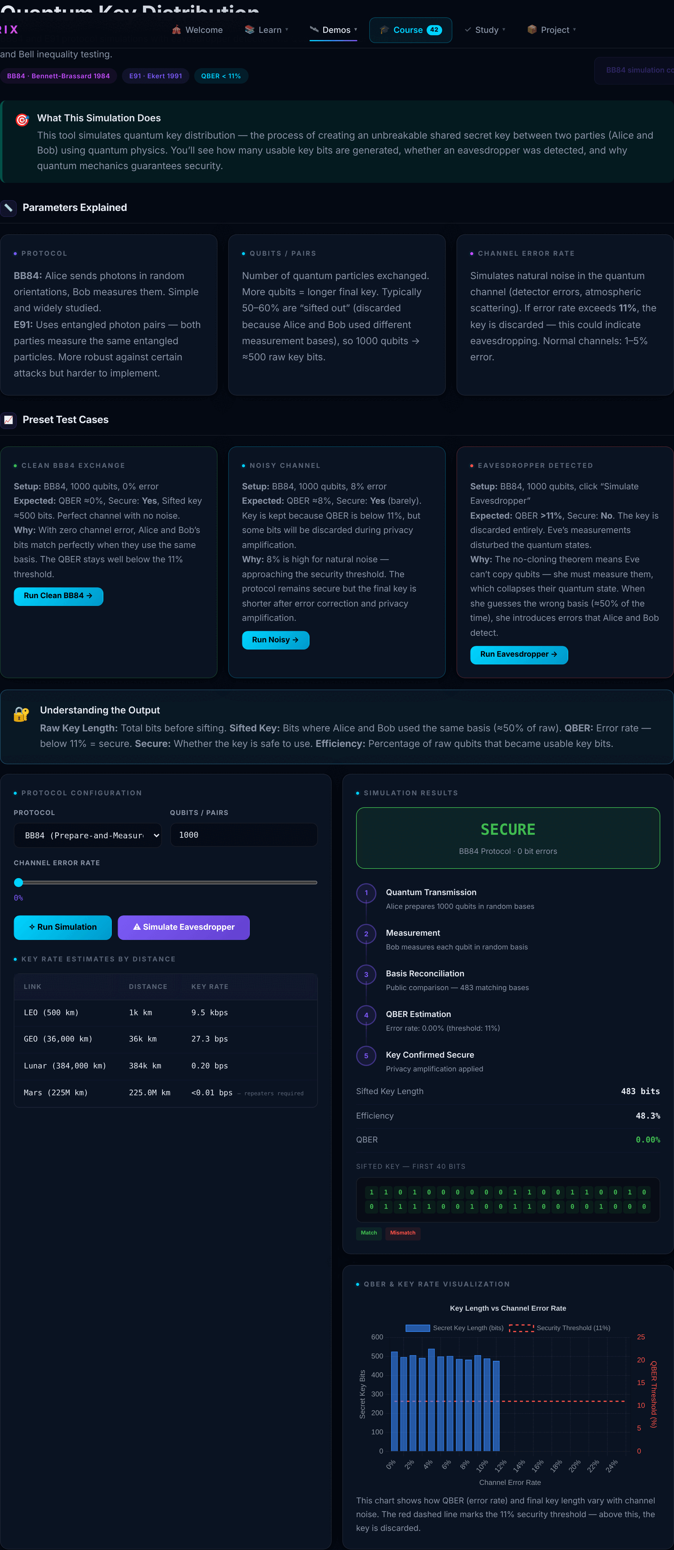
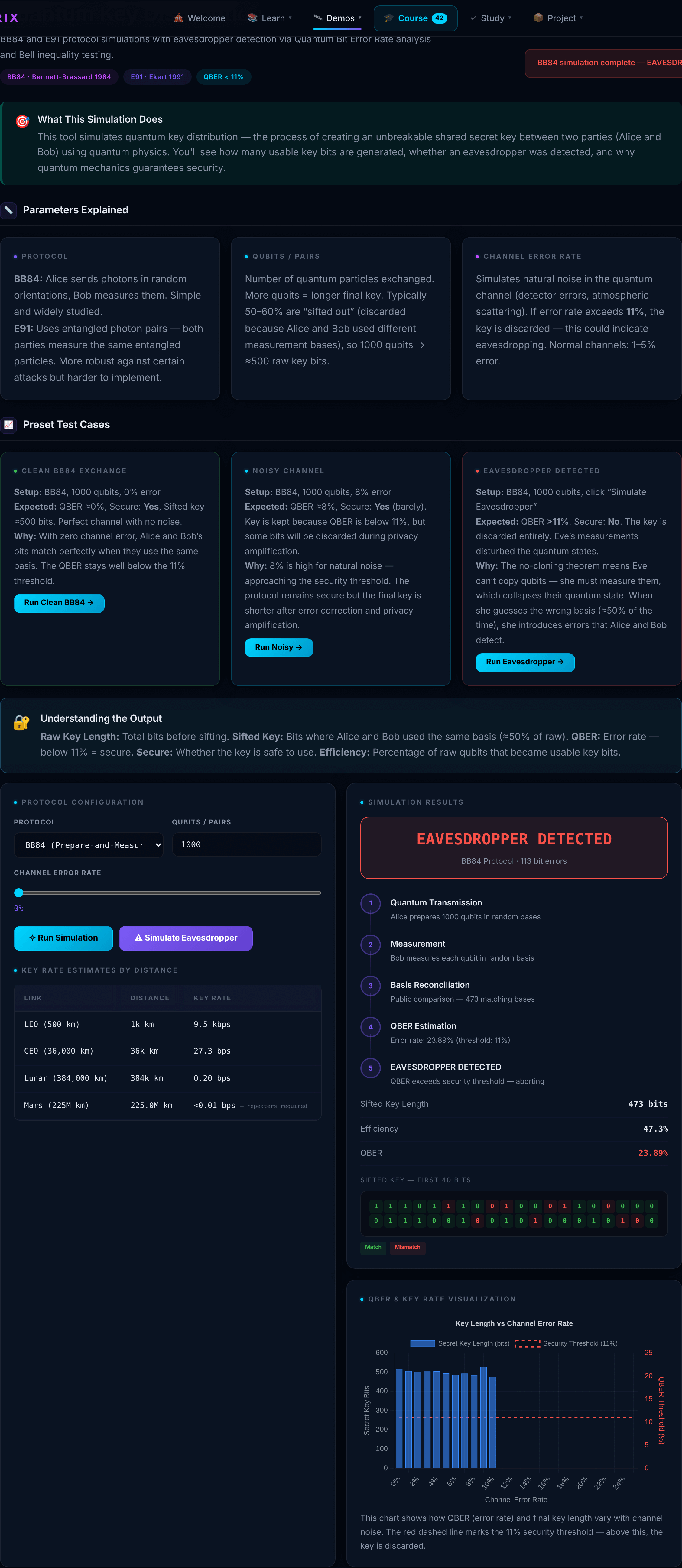
<0.01 bps — repeaters required. That collapse is 1/d² free-space diffraction loss, and it is the argument for entanglement-swapping repeaters on the interplanetary segment. It turns an apparent weakness into the justification for a design decision.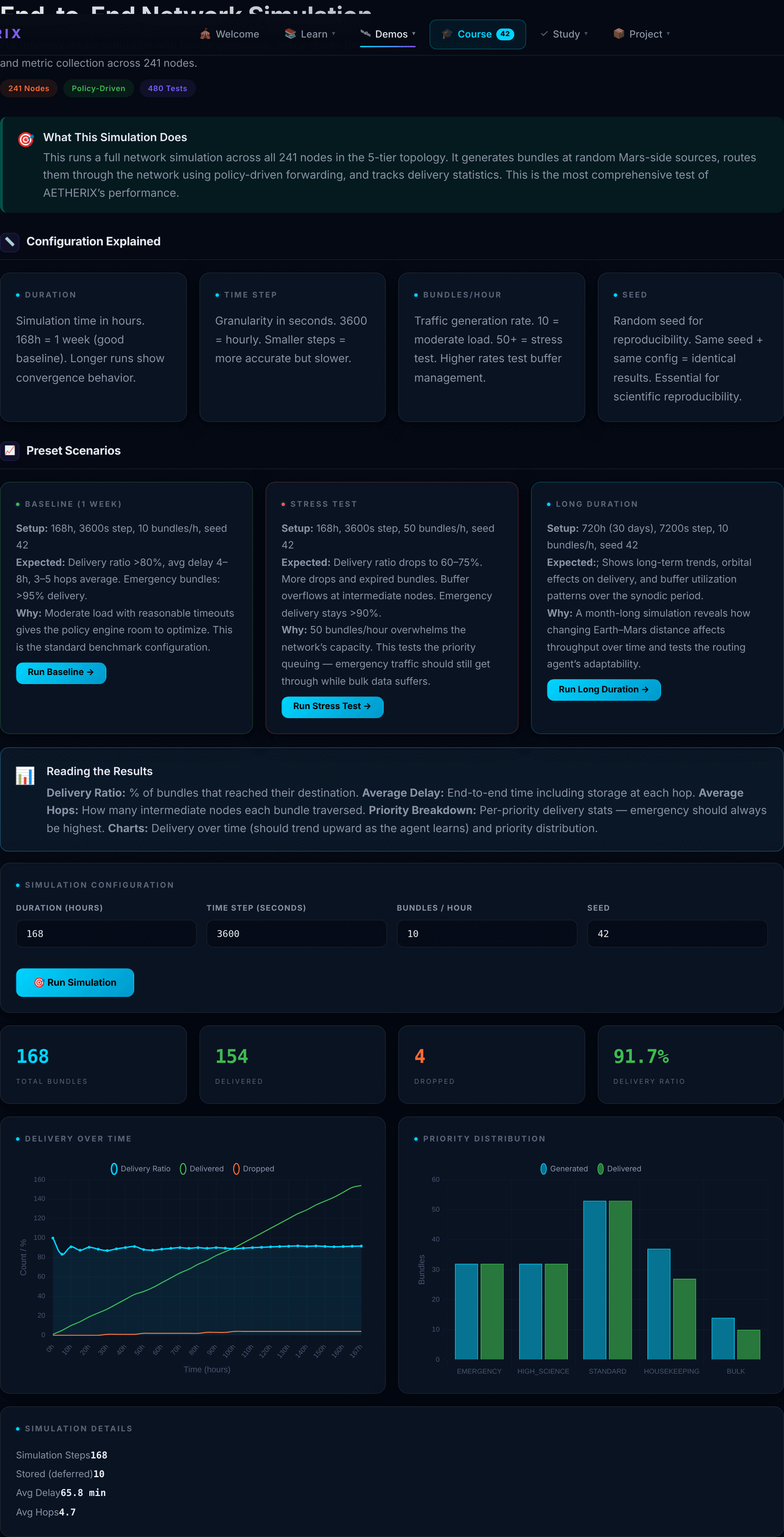
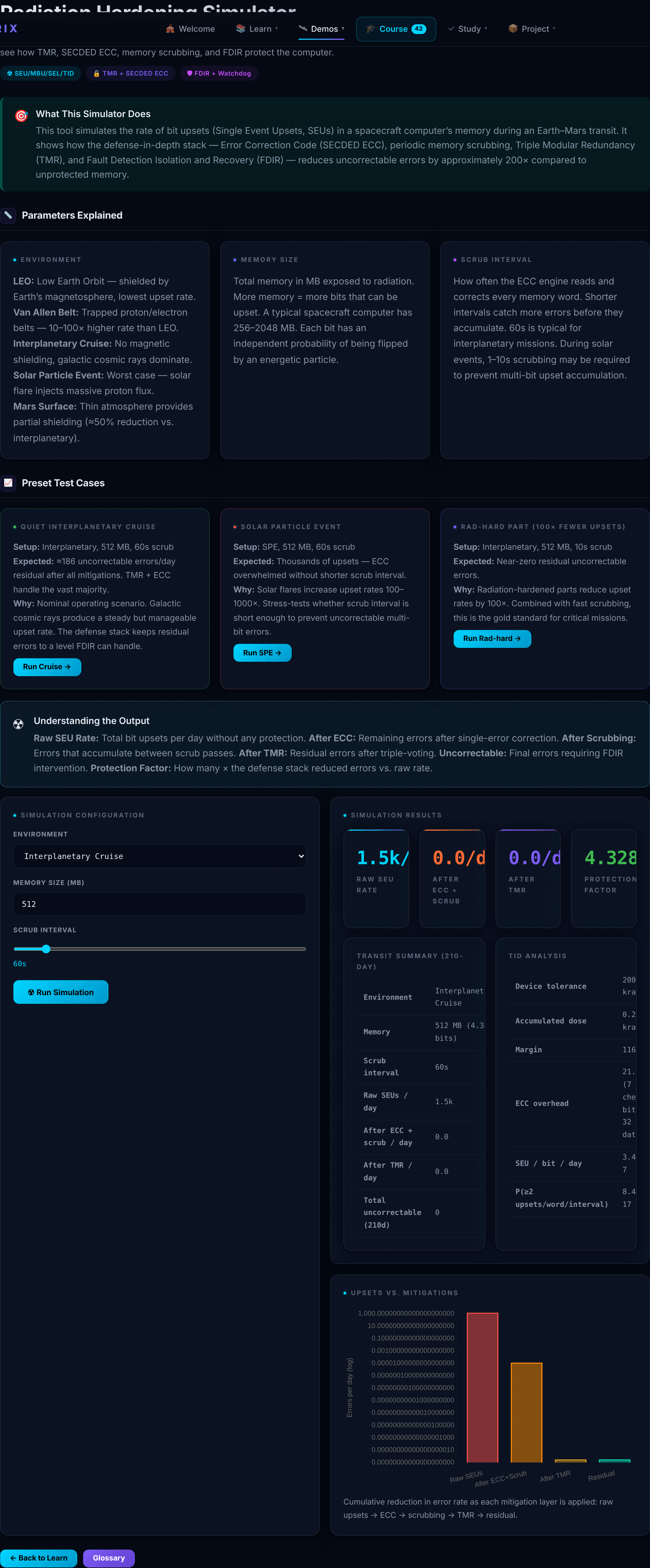
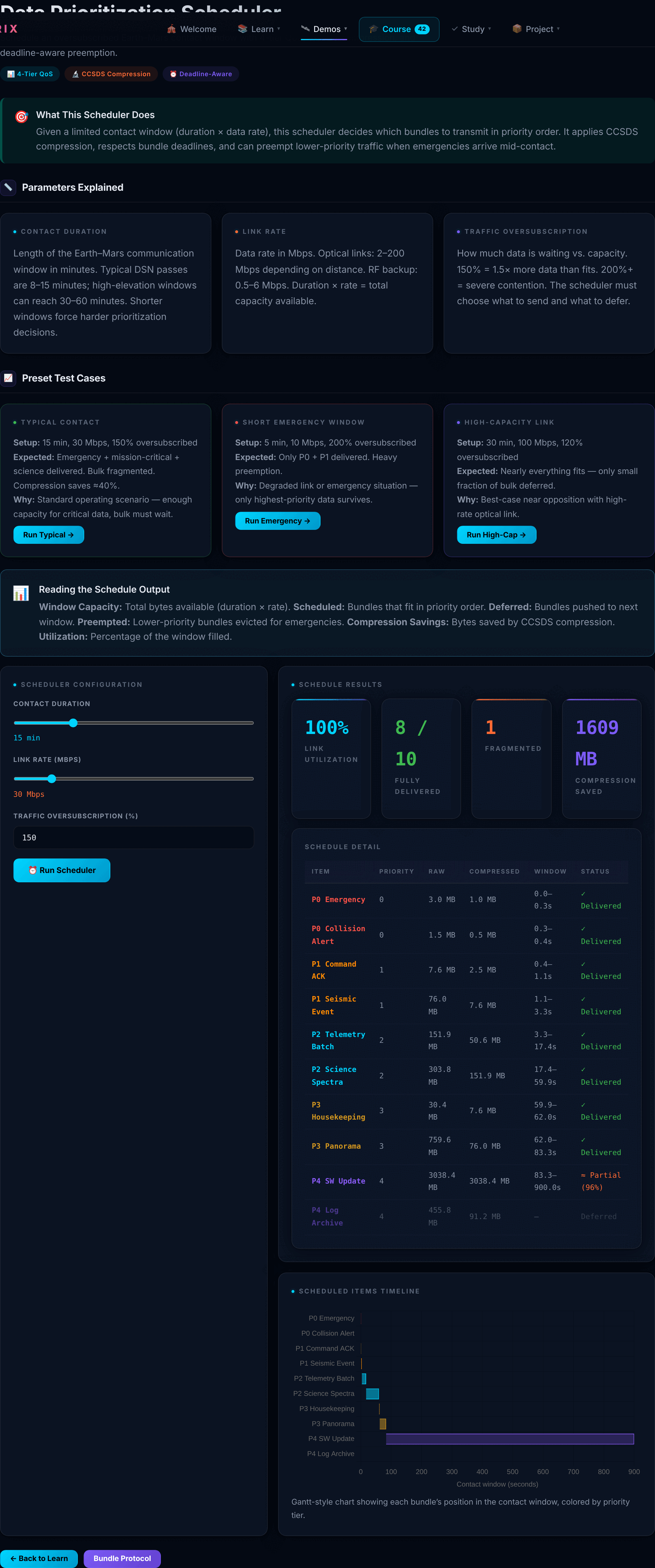
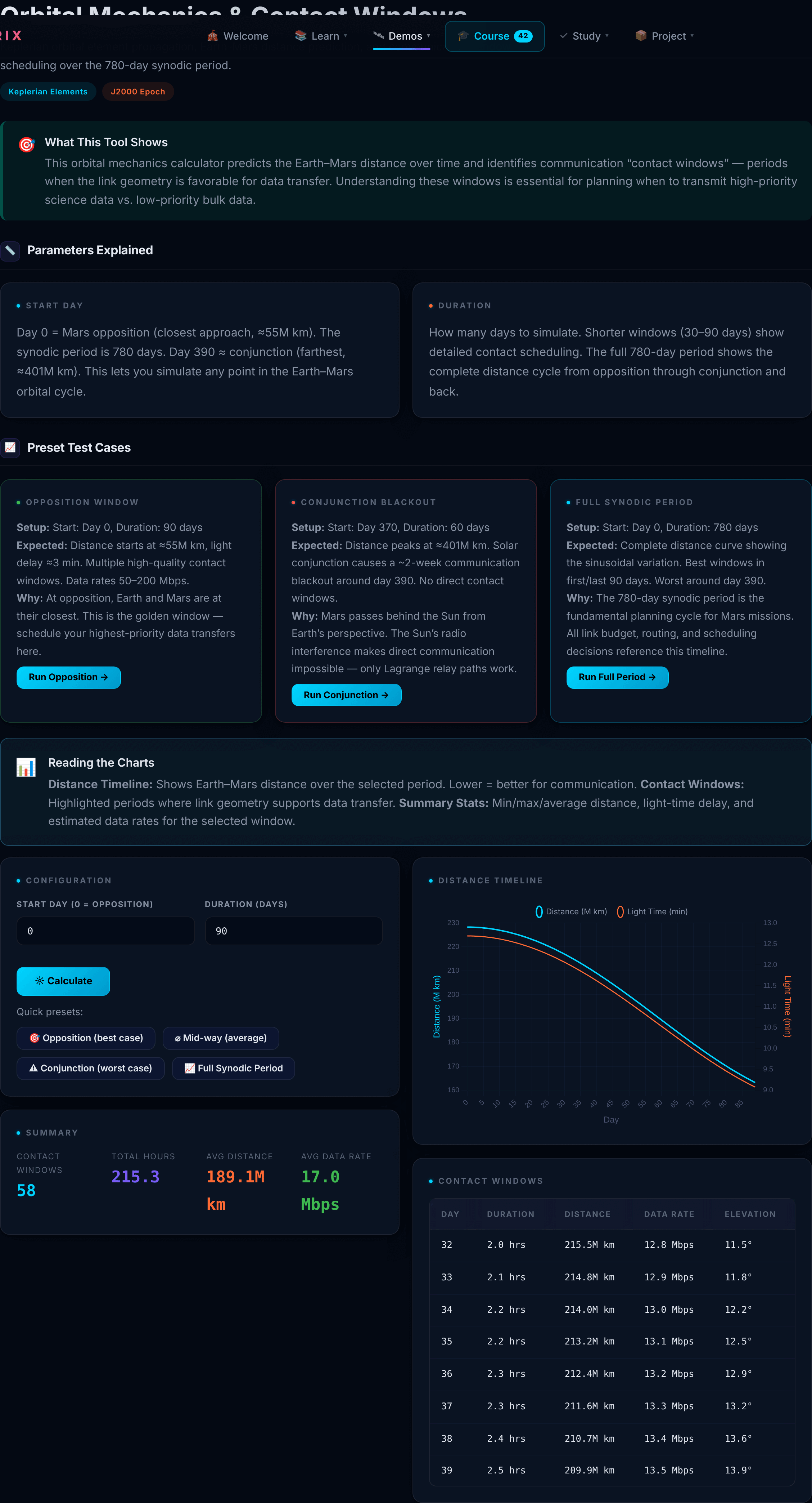
scheme://node/service form, priority class, lifetime, custody flag — and its routed path with per-hop actions.RL convergence is demonstrated; a head-to-head delivery-ratio benefit against a real ION-DTN CGR implementation is not. This is the biggest gap.
Closed by Phase 5–6
No SCPPM coding gain, no high-order PPM efficiency — roughly 13 dB conservative against the demonstrated DSOC point. Margins are a floor, not a rate prediction.
Closed by Phase 5–7
Its 31.9% delivery ratio must never be quoted as system performance. It exists so Module 3 has a “before” to improve on.
By design — not a gap
No generalisation to unseen states. Deliberate, for auditability — DQN is roadmap phase 6, labelled as future work rather than claimed.
Closed by Phase 6
Radiation figures are simulation outputs parameterised from published part characteristics, not irradiation testing.
Closed by Phase 7
No decoy states. A real weak-coherent-pulse source is vulnerable to the photon-number-splitting attack, which leaks key without raising QBER — so the current detection would miss it. The key-rate bound is also asymptotic, not finite-key.
Closed by Phase 8
Not JPL Horizons ephemeris. Good to a few percent; not mission-grade. Throughput and availability figures are targets, not measurements.
Closed by Phase 6
python run_simulation.py. Do not apologise twice and do not fix it live. Composure under a failed demo reads as engineering maturity.Mission Control Dashboard
Quick scenarios, distance timeline, and network topology overview.
Optical Link Budget Calculator
CCSDS 141.0-B-1 compliant deep-space optical link analysis at 1550 nm with free-space loss, antenna gain, and atmospheric attenuation modeling. Receiver sensitivity uses a photon-counting model identical to src/infrastructure/link_budget.py; it is uncoded, so it excludes SCPPM coding gain and high-order PPM efficiency (≈13 dB) and reports a conservative floor.
The Earth–Mars distance in millions of kilometers. This is the single biggest factor — signal strength drops with the square of the distance. Doubling the distance means 4× less signal (−12 dB).
Tx Power: Laser output in watts. More power = stronger signal. Typical: 1–10W for space lasers.
Tx Aperture: Telescope diameter on the transmitter side (meters). Larger = tighter beam = more gain at the receiver.
Rx Aperture: Receiver telescope diameter. DSN stations use 1–5m optical receivers.
Data Rate: Target speed in Mbps. Higher rates require more signal — there’s a trade-off between speed and distance.
Preset: Min 55M km, 5W, 0.22m Tx, 5.0m Rx, 2 Mbps
Expected: Link margin +4.31 dB — the link closes with headroom for atmospheric degradation, pointing error and ageing. Matches run_simulation.py Module 2 exactly.
Why: At 55M km, free-space loss is ≈−252 dB (vs −270 dB at max distance). This 18 dB advantage means the signal is 63× stronger than at conjunction.
Preset: Avg 225M km, 5W, 0.22m Tx, 5.0m Rx, 0.15 Mbps
Expected: Link margin +3.33 dB — positive but tight. Note the rate has dropped to 0.15 Mbps: at 4× the distance the budget buys rate down to keep the link closed.
Why: 225M km is 4× farther than opposition. Free-space loss increases by ≈12 dB — consuming most of the margin from the best case.
Preset: Max 401M km, 5W, 0.22m Tx, 5.0m Rx, 0.05 Mbps
Expected: Link margin +3.08 dB at 0.05 Mbps. Raise the rate back to 10 Mbps and the margin goes to −33.7 dB — that trade is the whole point of a link budget.
Why: At 390M km, free-space loss reaches ≈−269 dB. The signal is extremely weak — like seeing a candle on the Moon. This is where relay satellites become essential.
Reinforcement Learning Routing Agent
Q-learning based DTN routing with epsilon-greedy policy across a multi-tier interplanetary network topology.
Current Node: Where the bundle is right now. Options span all 5 tiers from Mars surface to Earth ground stations. The agent considers which neighbors are reachable from this node.
Destination: Where the bundle needs to go. The agent calculates the best path from current node to destination through the network.
Priority: EMERGENCY (0) through BULK (4). Emergency bundles force forwarding even on poor links. Bulk bundles may be stored until conditions improve.
Buffer Occupancy: How full the node’s storage is (0–100%). At >80%, the agent may drop low-priority bundles to make room for critical ones.
Setup: Node: mars.surface.rover-01, Dest: earth.control.moc, Priority: EMERGENCY, Buffer: 35%
Expected: Action: FORWARD immediately, even on marginal links. The agent prioritizes emergency delivery above all else — it will use any available path.
Why: Priority 0 overrides buffer and link quality concerns. Emergency data (solar flare alerts, system failures) cannot wait.
Setup: Node: transit.esl4.relay, Dest: earth.control.moc, Priority: STANDARD, Buffer: 90%
Expected: Action: STORE or cautious forward. With buffer nearly full, the agent may prefer to wait rather than risk a drop if the next hop can’t accept the bundle.
Why: At 90% buffer, the risk of overflow is high. Standard priority data can afford to wait for a cleaner transmission window.
Setup: Node: earth.leo.constellation, Dest: earth.control.moc, Priority: BULK, Buffer: 35%
Expected: Action: FORWARD or SPLIT. Low buffer pressure and proximity to destination allow the agent to route freely, potentially splitting for multipath delivery.
Why: LEO mesh has many paths to Earth ground. Bulk data benefits from multipath delivery — even if some fragments are lost, the total throughput is higher.
Quantum Key Distribution
BB84 and E91 protocol simulations with eavesdropper detection via Quantum Bit Error Rate analysis and Bell inequality testing.
BB84: Alice sends photons in random orientations, Bob measures them. Simple and widely studied.
E91: Uses entangled photon pairs — both parties measure the same entangled particles. More robust against certain attacks but harder to implement.
Number of quantum particles exchanged. More qubits = longer final key. Typically 50–60% are “sifted out” (discarded because Alice and Bob used different measurement bases), so 1000 qubits → ≈500 raw key bits.
Simulates natural noise in the quantum channel (detector errors, atmospheric scattering). If error rate exceeds 11%, the key is discarded — this could indicate eavesdropping. Normal channels: 1–5% error.
Setup: BB84, 1000 qubits, 0% error
Expected: QBER ≈0%, Secure: Yes, Sifted key ≈500 bits. Perfect channel with no noise.
Why: With zero channel error, Alice and Bob’s bits match perfectly when they use the same basis. The QBER stays well below the 11% threshold.
Setup: BB84, 1000 qubits, 8% error
Expected: QBER ≈8%, Secure: Yes (barely). Key is kept because QBER is below 11%, but some bits will be discarded during privacy amplification.
Why: 8% is high for natural noise — approaching the security threshold. The protocol remains secure but the final key is shorter after error correction and privacy amplification.
Setup: BB84, 1000 qubits, click “Simulate Eavesdropper”
Expected: QBER >11%, Secure: No. The key is discarded entirely. Eve’s measurements disturbed the quantum states.
Why: The no-cloning theorem means Eve can’t copy qubits — she must measure them, which collapses their quantum state. When she guesses the wrong basis (≈50% of the time), she introduces errors that Alice and Bob detect.
Orbital Mechanics & Contact Windows
Keplerian orbital element propagation, Earth-Mars distance prediction, and communication window scheduling over the 780-day synodic period.
Day 0 = Mars opposition (closest approach, ≈55M km). The synodic period is 780 days. Day 390 ≈ conjunction (farthest, ≈401M km). This lets you simulate any point in the Earth–Mars orbital cycle.
How many days to simulate. Shorter windows (30–90 days) show detailed contact scheduling. The full 780-day period shows the complete distance cycle from opposition through conjunction and back.
Setup: Start: Day 0, Duration: 90 days
Expected: Distance starts at ≈55M km, light delay ≈3 min. Multiple high-quality contact windows. Data rates 50–200 Mbps.
Why: At opposition, Earth and Mars are at their closest. This is the golden window — schedule your highest-priority data transfers here.
Setup: Start: Day 370, Duration: 60 days
Expected: Distance peaks at ≈401M km. Solar conjunction causes a ~2-week communication blackout around day 390. No direct contact windows.
Why: Mars passes behind the Sun from Earth’s perspective. The Sun’s radio interference makes direct communication impossible — only Lagrange relay paths work.
Setup: Start: Day 0, Duration: 780 days
Expected: Complete distance curve showing the sinusoidal variation. Best windows in first/last 90 days. Worst around day 390.
Why: The 780-day synodic period is the fundamental planning cycle for Mars missions. All link budget, routing, and scheduling decisions reference this timeline.
Bundle Protocol v7
RFC 9171 / CCSDS 734.2-B-1 compliant bundle creation, custody transfer, and multi-hop DTN routing visualization.
DTN Endpoint IDs in the format dtn://node/service. The source is where the bundle originates; the destination is the final recipient. The routing engine computes the multi-hop path between them.
Priority: EMERGENCY (0) — life-safety alerts. BULK (4) — archive dumps. Determines queuing order at each hop.
Payload: The actual data in MB. Bundles can carry up to GBs — millions of times larger than TCP packets.
Deadline: Hours until the bundle must arrive. Expired bundles are dropped to free buffer space.
Lifetime: Maximum days the bundle can exist in the network. Prevents stale data from circulating forever in a DTN.
Setup: Rover → Earth MOC, EMERGENCY, 1 MB, 4h deadline
Expected: Immediate forwarding through all hops. Custody transfer at every node. Priority 0 means it jumps to the front of every queue.
Why: Small payload + highest priority + short deadline = fastest possible delivery. Think solar flare warning or system failure alert.
Setup: Rover → Earth MOC, STANDARD, 500 MB, 168h deadline
Expected: Standard queuing at each hop. May be stored at intermediate nodes during unfavorable contact windows. 7-day deadline allows flexible routing.
Why: 500 MB of science data can tolerate delays. The routing agent will choose energy-efficient paths and wait for good contact windows.
Setup: Earth DSN → Mars Areo, BULK, 2000 MB, 720h deadline
Expected: Lowest priority in every queue. Sent during off-peak windows when no higher-priority data is waiting. 30-day lifetime accommodates slow delivery.
Why: Software updates are large but not time-critical. The network fills spare capacity with bulk data, maximizing throughput without impacting operations.
DTN Store-and-Forward Engine
Full Bundle Protocol v7 forwarding engine with priority queuing, LTP convergence layer, custody transfer, and policy-driven routing across the 241-node topology.
The bundle payload in bytes. LTP breaks large payloads into segments that fit the link MTU. Larger payloads = more segments = more chances for loss, but also more efficient use of the link.
The largest single segment that can be sent in one frame. Smaller MTU = more segments = more overhead but finer-grained retransmission. Deep-space links typically use 1400 bytes.
Percentage of segments lost in transit (simulates atmospheric interference, pointing errors). LTP selectively retransmits only lost segments — not the entire payload. Critical for 20+ minute delay links.
Setup: 10000 bytes, 1400 MTU, 0% loss
Expected: 8 segments sent, 8 received. Zero retransmissions. Total transfer time = 1 round trip.
Why: With no loss, LTP is a simple segmentation protocol — split, send, acknowledge. The ideal baseline case.
Setup: 10000 bytes, 1400 MTU, 5% loss
Expected: ≈1 segment lost on average. LTP retransmits only the lost segment. Total transfer time ≈2 round trips.
Why: At 5% loss, roughly 1 in 20 segments is lost. LTP’s selective retransmission is far more efficient than TCP’s go-back-N approach over 20-minute-delay links.
Setup: 100000 bytes, 1400 MTU, 20% loss
Expected: ≈72 segments, ≈14 lost. Multiple retransmission rounds required. Transfer time ≈3–4 round trips.
Why: At 20% loss, the link is severely degraded (solar storm scenario). LTP still delivers — eventually — because each retransmission round only resends what was lost, not everything.
RF Link Budget Calculator
Ka-band, X-band, S-band, and UHF link budget analysis for hybrid optical/RF Earth-Mars communication (CCSDS 401.0-B-30).
Ka-band (26.5 GHz): Highest RF data rate but weather-sensitive. X-band (8.4 GHz): Current Mars standard — reliable, moderate speed. S-band (2.3 GHz): Command uplink. UHF (401 MHz): Mars surface-to-orbiter short range.
Antenna diameter in meters. Larger dishes = higher gain = longer range. Spacecraft typically have 1–5m dishes; DSN ground stations have 34–70m dishes. Gain increases with frequency and dish size.
Tx Power: Transmitter output in watts. Spacecraft: 5–40W. Ground: up to 400W.
Data Rate: Target speed in bps. RF is much slower than optical: typical 1 kbps–6 Mbps vs optical’s 2–200 Mbps.
| Property | Optical (1550nm) | Ka-band RF | X-band RF |
|---|---|---|---|
| Wavelength | 1550 nm | 11.3 mm | 35.7 mm |
| Beam Divergence | ≈5 μrad (very narrow) | ≈0.5 mrad | ≈1.5 mrad |
| Data Rate | 2–200 Mbps | 1–50 Mbps | 0.5–6 Mbps |
| Weather Immunity | Low (clouds block) | Moderate (rain fade) | High |
| Best For | Bulk science downlink | High-rate backup | Reliable command/telemetry |
Setup: Ka-band, 225M km, 20W, 3m/34m dishes, 1 Mbps
Expected: Link margin +2 to +6 dB. Reliable high-rate downlink for bulk science data at average distance.
Why: This is the baseline Ka-band scenario for Mars relay operations, representing typical operating conditions.
Setup: X-band, 225M km, 10W, 2m/34m dishes, 256 kbps
Expected: Link margin +8 to +15 dB. Very robust link for commanding, telemetry, and safe-mode operations.
Why: X-band is the reliable fallback when Ka-band is weather-impacted or during safe-mode. Lower data rate but very high margin.
Setup: UHF, 0.02M km (20km), 5W, 0.1m/0.5m antennas, 128 kbps
Expected: Link margin +15 to +25 dB. Short-range surface-to-orbiter link for rover and habitat communications.
Why: UHF fills the last-mile gap on Mars — connecting surface assets to orbiting relays. Very short range but sufficient for local networks.
End-to-End Network Simulation
Full topology-aware simulation with bundle generation, policy-driven forwarding, multi-hop routing, and metric collection across 241 nodes.
Simulation time in hours. 168h = 1 week (good baseline). Longer runs show convergence behavior.
Granularity in seconds. 3600 = hourly. Smaller steps = more accurate but slower.
Traffic generation rate. 10 = moderate load. 50+ = stress test. Higher rates test buffer management.
Random seed for reproducibility. Same seed + same config = identical results. Essential for scientific reproducibility.
Setup: 168h, 3600s step, 10 bundles/h, seed 42
Expected: Delivery ratio >80%, avg delay 4–8h, 3–5 hops average. Emergency bundles: >95% delivery.
Why: Moderate load with reasonable timeouts gives the policy engine room to optimize. This is the standard benchmark configuration.
Setup: 168h, 3600s step, 50 bundles/h, seed 42
Expected: Delivery ratio drops to 60–75%. More drops and expired bundles. Buffer overflows at intermediate nodes. Emergency delivery stays >90%.
Why: 50 bundles/hour overwhelms the network’s capacity. This tests the priority queuing — emergency traffic should still get through while bulk data suffers.
Setup: 720h (30 days), 7200s step, 10 bundles/h, seed 42
Expected:; Shows long-term trends, orbital effects on delivery, and buffer utilization patterns over the synodic period.
Why: A month-long simulation reveals how changing Earth–Mars distance affects throughput over time and tests the routing agent’s adaptability.
Integrated Mars Mission Scenario
End-to-end simulation combining link budget analysis, RL routing, quantum key distribution, orbital mechanics, and bundle protocol in a single mission scenario.
Day 0 = Mars opposition. Day 390 = conjunction. This sets the initial Earth–Mars distance and orbital geometry, which affects link budgets throughout the simulation.
Mission duration in days. 30 days = one contact window. 90 days = seasonal planning. 365 days = full mission phase showing distance variation.
Number of bundles generated for each priority level (5 levels). Total bundles = 5 × this number. 25 = 125 total bundles (moderate). 100 = 500 bundles (stress test).
Setup: Start Day 0, 30 days, 25 bundles/type
Expected: High throughput, low latency. QKD key rate — 5–10 kbps. Delivery ratio >90%. This is the best-case mission scenario.
Why: Opposition gives the shortest distance, strongest signal, and fastest data rates. Mission planners concentrate high-priority science observations for this window.
Setup: Start Day 370, 60 days, 25 bundles/type
Expected: Reduced throughput, some blackouts. Lagrange relays maintain partial connectivity. QKD key rate drops significantly. Emergency delivery remains >80%.
Why: This stress-tests the network’s resilience during the worst orbital conditions. The RL routing agent must find alternative paths through relays.
Setup: Start Day 0, 365 days, 15 bundles/type
Expected:; Shows the full performance envelope — from peak throughput at opposition through the conjunction bottleneck and back. Reveals seasonal patterns in delivery statistics.
Why: A full year captures the complete range of operating conditions. This is the scenario used for long-term mission planning and infrastructure sizing.
Radiation Hardening Simulator
Simulate the impact of space radiation on spacecraft electronics during an Earth–Mars transit, and see how TMR, SECDED ECC, memory scrubbing, and FDIR protect the computer.
LEO: Low Earth Orbit — shielded by Earth’s magnetosphere, lowest upset rate.
Van Allen Belt: Trapped proton/electron belts — 10–100× higher rate than LEO.
Interplanetary Cruise: No magnetic shielding, galactic cosmic rays dominate.
Solar Particle Event: Worst case — solar flare injects massive proton flux.
Mars Surface: Thin atmosphere provides partial shielding (≈50% reduction vs. interplanetary).
Total memory in MB exposed to radiation. More memory = more bits that can be upset. A typical spacecraft computer has 256–2048 MB. Each bit has an independent probability of being flipped by an energetic particle.
How often the ECC engine reads and corrects every memory word. Shorter intervals catch more errors before they accumulate. 60s is typical for interplanetary missions. During solar events, 1–10s scrubbing may be required to prevent multi-bit upset accumulation.
Setup: Interplanetary, 512 MB, 60s scrub
Expected: ≈186 uncorrectable errors/day residual after all mitigations. TMR + ECC handle the vast majority.
Why: Nominal operating scenario. Galactic cosmic rays produce a steady but manageable upset rate. The defense stack keeps residual errors to a level FDIR can handle.
Setup: SPE, 512 MB, 60s scrub
Expected: Thousands of upsets — ECC overwhelmed without shorter scrub interval.
Why: Solar flares increase upset rates 100–1000×. Stress-tests whether scrub interval is short enough to prevent uncorrectable multi-bit errors.
Setup: Interplanetary, 512 MB, 10s scrub
Expected: Near-zero residual uncorrectable errors.
Why: Radiation-hardened parts reduce upset rates by 100×. Combined with fast scrubbing, this is the gold standard for critical missions.
Data Prioritization Scheduler
Schedule an oversubscribed Earth–Mars contact window with 4-tier QoS, CCSDS compression, and deadline-aware preemption.
Length of the Earth–Mars communication window in minutes. Typical DSN passes are 8–15 minutes; high-elevation windows can reach 30–60 minutes. Shorter windows force harder prioritization decisions.
Data rate in Mbps. Optical links: 2–200 Mbps depending on distance. RF backup: 0.5–6 Mbps. Duration × rate = total capacity available.
How much data is waiting vs. capacity. 150% = 1.5× more data than fits. 200%+ = severe contention. The scheduler must choose what to send and what to defer.
Setup: 15 min, 30 Mbps, 150% oversubscribed
Expected: Emergency + mission-critical + science delivered. Bulk fragmented. Compression saves ≈40%.
Why: Standard operating scenario — enough capacity for critical data, bulk must wait.
Setup: 5 min, 10 Mbps, 200% oversubscribed
Expected: Only P0 + P1 delivered. Heavy preemption.
Why: Degraded link or emergency situation — only highest-priority data survives.
Setup: 30 min, 100 Mbps, 120% oversubscribed
Expected: Nearly everything fits — only small fraction of bulk deferred.
Why: Best-case near opposition with high-rate optical link.
Why This Over That
Every architecture choice in AETHERIX was made against a concrete alternative. Here is the reasoning, trade-off by trade-off — the section an examiner should start with.
Why: TCP’s three-way handshake and congestion control assume round-trip times below the retransmission-timeout floor. At 3–22 minutes of one-way light delay, a TCP session across the Earth–Mars gap is mathematically incapable of staying up, and continuous end-to-end connectivity never exists. BPv7’s store-carry-forward custody model (RFC 9171) moves the reliability unit from the link to the bundle, so a partitioned network still delivers. Why not TCP/IP: it is the right tool for the Earth and Mars local segments — and AETHERIX uses it exactly there (TCPCL, RFC 7242) — but not for the interplanetary backbone.
Why: 1550 nm optical offers 10–100× the bandwidth of Ka-band at the same mass budget, but optical links die in clouds, dust, and solar-conjunction geometry; Ka/X-band RF survives them at lower rate. A hybrid terminal gets optical’s throughput with RF’s availability. Why not single-mode: optical-only forfeits conjunction-season communications entirely (see the solar_conjunction scenario’s RF-fallback behaviour); RF-only caps the science return by an order of magnitude.
Why: 1550 nm rides the mature fibre-telecom component ecosystem — InGaAs detectors, telecom-grade amplifiers, WDM-quality optics — sits in a clean atmospheric transmission window, and is the band NASA’s own lunar lasercom demonstrations used. The honest trade: for a fixed aperture, a shorter wavelength actually diffracts less — 850 nm would give a tighter beam — but you would trade into a component desert: no flight-qualified amplifier chain, no detector ecosystem, worse receiver sensitivity in practice. The optics supply chain is part of the link budget.
Why: each segment’s physics picks its transport. The Earth segment (milliseconds, wired) runs TCPCL (RFC 7242) where TCP’s ecosystem of TLS and middleboxes wins. The deep-space hop runs LTP (RFC 5326), whose checkpoint-based selective ARQ was engineered for minutes-long delays — no handshake, no ACK clock. The laser crosslinks run UDPCL with fragmentation, because an ISL has no congestion, only loss. Why not one transport: every candidate fails somewhere — TCP dies at light-time, LTP over a LAN is wasted machinery, bare UDP has no reliability at all.
Why: an end-to-end acknowledgment across Earth–Mars costs a 6–44 minute round trip — the sender stalls for the better part of an hour per loss. DTN custody (CCSDS 734.2-B-1 §3 + Annex D) moves the retransmission duty hop-by-hop: each relay accepting custody re-sends only over its own short-delay link, and buffer space becomes the network’s currency. Why not end-to-end: it treats a 2-hop and a 20-hop path identically and pays full light-time for every recovery — through a network whose whole point is that the path is long.
Why: OSPF-style protocols compute paths over a connected snapshot of the topology; the interplanetary graph is disconnected most of the time — an edge exists only inside a scheduled contact window. AETHERIX routes over the (node, time) contact graph (contact_graph.py): pathfinding only through contacts that are actually open at forwarding time. Why not link-state: a table computed on “connected now” would be empty for hours at a stretch, and one computed on “eventually connected” hands bundles to voids.
Why: in a 2 Mbps conjunction-season window, an EMERGENCY telecommand and a bulk terrain map cannot politely share a queue — one of them is worthless if late. Bundles carry one of five BPv7 priority classes (EMERGENCY…BULK), and the scheduler orders within each class by deadline, preempting bulk for time-critical traffic (prioritization.py). Why not FIFO: it is trivially fair and trivially wrong — fair to the data, not to the mission.
Why: CGR (CCSDS 734.3-B-1) computes best routes from a pre-planned contact schedule — optimal while the plan holds, brittle the moment it doesn’t. A dust storm delays a rover, a relay drops to safe mode, and the graph no longer matches reality. An RL agent that observes link quality, buffer occupancy, and bundle deadlines keeps making the best available decision, and the reward function R = α(delivery) − β(delay) − γ(hops) − δ(drops) − ε(energy) encodes the mission’s actual trade-offs. Why not pure CGR: the DSN runs on schedules today, so AETHERIX’s policy engine ships CGR-style rule policies as the fallback tier — RL earns its keep in the disrupted cases the schedule can’t see.
Why: the state space is genuinely discrete — a 5-tier topology, bounded link-quality and buffer bins, five priorities, four actions — which is exactly the regime where a Q-table is the theoretically correct estimator, not a compromise. The learned policy can be printed and inspected cell-by-cell, every number is reproducible from a seed with zero external dependencies, and convergence is detectable by auditing the table’s deltas. Why not a DQN: deep networks pay off in continuous, high-dimensional spaces; here they would add a 2 GB dependency, version pinning, seed-sensitive training runs, and a black box in front of the exact quantities an examiner asks about (reward shaping, ε-decay, convergence). A DQN upgrade path exists in the roadmap — it is a deliberate later, not a miss.
Why: the autonomy loop’s detector (src/simulation/anomaly.py) maintains per-node, per-metric EWMA baselines and flags ≥2 metrics simultaneously beyond 3.5σ. It is unsupervised (no labelled training set to drift out of date), explainable (every alarm cites its z-scores), self-limiting (anomalous samples never update the baseline, so an attack cannot poison its own detector), and deterministic stdlib. Why not a neural classifier: a supervised model trained on simulated attacks learns the simulator’s fingerprints rather than the physics, invites label leakage (severity or source fields derived from the ground-truth label sneaking in as features), and turns every “why did it fire?” question into an archaeology dig through weights. Detection here must be auditable at 3–22 minutes of light distance.
Why: the telemetry generator couples link margin and data rate to Earth–Mars distance through the orbital module (inverse-square law) and models each anomaly as a physically consistent signature — link degradation collapses margin, a custody storm fills buffers, radiation corruption spikes checksum failures while the link stays healthy, and a navigation spoof (POSITION_SPOOF) drives the reported-vs-ephemeris position error to thousands of km while every RF/optical observable stays healthy — the exact mismatch an onboard ephemeris cross-check would catch, mitigated by EPHEMERIS_CROSSCHECK + NAV_QUARANTINE. A detector can only be honestly evaluated against telemetry that behaves like physics. Why not uniform random features: any classifier looks good against white noise; the scientific-strictness rule (cite the sample, the seed, the config — no fabricated numbers) starts with the generator.
Why: an RL agent explores by design — and the day it explores badly is the day an EMERGENCY bundle meets a full buffer. The policy engine ships five deterministic rule policies as the guaranteed-safe tier (policy_engine.py); the learned policy earns discretion inside the envelope the rules allow. Why not pure RL: an untrained or drifting agent is a single point of behavioural failure; deterministic rules are auditable line-by-line before launch and boring in exactly the way safety-critical software should be.
Why: no Mars asset can stream gradients to an Earth learner at 3–22 minutes of light time — and back. Agents train locally on the traffic they actually see and merge Q-tables opportunistically when contacts allow (multi_agent.py) — the same delay-tolerant store-and-poll trick the network itself uses for data, applied to learning. Why not centralized: the training round-trip would be slower than the mission, and the central model would never see the local conditions (buffer pressure, link quality) each node actually routes under.
Why: plain averaging is optimal only when every contributor is honest — but a single compromised or corrupted relay contributing a poisoned Q-table shifts the mean arbitrarily. The coordinator’s coordinate-wise median tolerates up to just-under-half Byzantine contributors, and trimmed mean (dropping each cell’s min/max) suits small contributor counts; rounds also proceed with whoever shows up, because a federation that blocks on a relay behind the Sun never completes a round at all. Why not FedAvg: its robustness assumption (honest majority and full participation) is exactly what a 241-node network under attack and conjunction cannot promise.
Why: the first EWMA breach of an episode raises only a WATCH — raise sampling cadence, cross-validate against the node’s own baseline — and the full mitigation playbook fires only on a persistent breach (deployed at persistence = 2). In a sparse DTN topology, wrongly isolating a healthy relay (purging its custody refs, deferring its bulk traffic) costs real science return; a proportional response prices that in. Why not fire everything on first alarm: a detector with a nonzero false-positive rate plus an irreversible playbook is a system that cries wolf — and operators learn to ignore it, which is its own security failure.
Why: every intelligence dependency has a designed-in dumb fallback: an unconverged RL agent hands routing to the deterministic policy tier; a compromised or exhausted QKD pool drops security to classical hash-based mode; an unreachable audit sink spills to a bounded local buffer with a counted drop-oldest policy. Every switch is an audited event with a reason string (degradation.py). Why not let the smart part be load-bearing: the RL agent explores by design and the quantum channel has bad days; a network where “the AI is down” means “routing is down” has built its fragility in on purpose.
Why: link-quality observations decay exponentially with a configurable half-life (pheromone evaporation, contact_quality.py): fresh mediocrity outranks stale excellence by construction, and fully decayed memory falls back to the configured default — old news becomes ignorance, not pessimism. Why not a running average: an average over a link that was excellent before a conjunction and is dead after it will keep recommending a corpse for as long as the good samples outnumber the bad; decay forgets on a timescale you choose.
Why: each incident record commits cryptographically to its predecessor, so any retroactive edit — an attacker scrubbing their custody flood from history, or an operator quietly rewriting a response — breaks the chain, and verify_audit_chain() says exactly where. The same hash-chaining idea that makes blockchains append-only, applied to an operations log, at the cost of one SHA-256 per record. Why not a plain append-only file: “append-only” is a convention, not a property — nothing in a text log detects the line that was edited in place after the fact. If the audit record of an autonomous system can be silently rewritten, the autonomy has no accountability.
Why: the trainer stops when Q-value deltas fall below a criterion, not after an arbitrary N episodes (training.py) — so “converged” is a measured property, and every reported learning curve cites both the episode count and the gate that ended it. Why not fixed budgets: too few episodes hides non-convergence behind a clean-looking curve; too many burns compute and invites overfitting to simulator quirks — either way the number you quote is about the budget, not the agent.
Why: mission data must stay confidential for decades — an adversary can record ciphertext today and decrypt it once quantum hardware matures (“harvest now, decrypt later”). BB84/E91 key distribution is secured by physics (no-cloning, measurement disturbance), not by computational hardness, and eavesdropping raises QBER above the 11% Csiszár–Körner threshold where the key is simply discarded. Why not QKD alone: it needs line-of-sight quantum channels and only distributes keys — it neither authenticates nor survives a conjunction blackout — which is exactly why the integrity layer below exists.
Why hash-based (Lamport + Merkle): security reduces to SHA-256’s collision resistance — Shor’s algorithm simply has no structure to attack, and Grover only halves the exponent — while verification is pure hashing, cheap enough for flight avionics doing per-bundle checks on the store-and-forward path. Why not RSA/ECC: both collapse under Shor; signing long-lived mission profiles with them is a dated-lock on the door. Why not ML-DSA (FIPS 204) here: lattice-based NIST standards are the right production choice, but their lattices and Fiat-Shamir layers are far harder to audit line-by-line than 256 hash comparisons; the hash-based family (Lamport 1979, Merkle 1979 — the same family NIST standardised as SPHINCS+/FIPS 205) demonstrates the identical post-quantum property with an implementation an examiner can read in one sitting.
Why: QKD delivers information-theoretic symmetric keys but cannot authenticate bundles or operate without a quantum channel; hash-based signatures authenticate anywhere, anytime, but rest on computational (quantum-hard) assumptions. Layered, each covers the other’s blind spot: keys from physics, integrity from hashing. Why not pick one: every real interplanetary security architecture (e.g. NASA’s DTN PKI studies) layers; a single-mechanism answer is the wrong answer for a 20-year mission.
Why: every signature names its algorithm, unknown IDs fail closed, and each run emits a cryptographic bill of materials — algorithms, key/sizes, quantum assumptions, rotation policy, and the registered upgrade path (ML-DSA-65, SPHINCS+-128s). A 20-year mission will outlive at least one cryptographic fashion; agility is the field that lets it negotiate. Why not hardcode today’s choice: “we’ll migrate later” without a negotiation field and an inventory is a wish, not a plan — and the byte-cost of security stays invisible until it eats a 2 Mbps conjunction-season link.
Why: in a reproducible research codebase, even key material must be regenerable — CI regenerates the keyring from a seed every build and asserts the verification chain end-to-end, so a security regression fails the pipeline, not the mission. Why not CSPRNG everywhere: production signing would, obviously, use os.urandom() — the module supports it (pass seed=None) — but unsaved random keys make test failures un-reproducible. The demo keys sign demo bundles; nothing here pretends otherwise.
Why: direct single-photon exchange across 54.6–401 million km is beyond any realistic channel budget — the key rate collapses with distance no matter the engineering. The chain swaps entanglement hop-by-hop at Lagrange relays and purifies each pair before swapping, explicitly trading rate for fidelity (repeater_chain.py). Why not single-hop: the physics forbids it, not the budget — which is precisely why the relay tier exists in the topology at all.
Why: a sifted BB84 key still leaks information proportional to the QBER. CASCADE reconciliation repairs Alice/Bob discrepancies, then universal-hash privacy amplification compresses exactly the leakable fraction back out — bounded by the Csiszár–Körner result, which is also where the 11% abort threshold comes from: a theory-derived constant, not a tuned hyperparameter (privacy_amplification.py). Why not raw sifted keys: the “secure” flag would be marketing — the same physics that detects Eve also quantifies her, and only amplification spends that knowledge.
Why: TMR outvotes computation faults, SECDED ECC fixes single-bit memory errors, scrubbing prevents a second fault accumulating in the same word, and FDIR bounds whatever survives — each layer exists because the layer above it has a measurable residual (~200× combined reduction; see Radiation Hardening). Why not one silver bullet: every individual mitigation has a failure mode the others catch; a single mechanism is a single point of failure with a cosmic-ray trigger.
Why: autonomy needs a floor. The FDIR controller has a bounded recovery budget — reset, reload golden image, retry — and when it is exhausted, the node drops to a minimal-power SAFE-MODE and waits for ground (radiation.py). Why not recover forever: an agent that never gives up can thrash indefinitely on an unfixable fault, draining power and corrupting state; knowing when to stop and phone home is itself a reliability feature — the same philosophy behind the deterministic policy fallback in routing.
Why: every module under src/ runs on a bare Python 3.9+ interpreter — clone, python src/simulation/telemetry.py, done. Zero pinned dependencies means zero version-drift failures and identical numbers on any machine, forever. Why not heavy frameworks: framework convenience is paid for in reproducibility, install time, and auditability; the core’s math (link budgets, orbital mechanics, EWMA, hash chains) needs no linear algebra library. External deps live where they earn their keep — FastAPI for the API surface — and nowhere else.
Why: the pipeline gates what ships, not what looks good: the security chain (sign → verify → tamper/replay rejected) must pass on every build; the autonomy ladder must hold its measured precision/detection/FP budgets across fixed seeds; and a known-event regression reruns the seeded solar-conjunction blackout asserting delivery survives, accounting stays physical, and two runs produce identical numbers. Why not manual review: security and quality properties decay silently; only an executable check that runs on every commit catches the regression the day it lands rather than the week before launch.
Why: nothing propagates faster than c, margins/rates/temperatures stay in mission-class domains, contacts never overlap a blackout, and accounting identities hold — enforced by code (plausibility.py) that runs in CI behind every published figure. Why not eyeball the outputs: the failure mode of a simulation is a plausible-looking number that is physically impossible; guards turn that from a review-time argument into a build failure. This is also the discipline that separates a measured 3.5% conjunction-season delivery ratio from a slide that says “99.9% uptime”.
Why: POST /api/telemetry/stream recomputes the entire run from its seed instead of storing rows — what happened and what is stored cannot diverge, and the audit of any result is simply “re-run it”. Why not a telemetry database: persisted streams invite silent drift (schema changes, physics changes, pruned rows), and a stored anomaly that can’t be regenerated is indistinguishable from a bug. Stateless request/response also keeps every response a citable artifact — the same reason a streaming command endpoint was removed earlier in the project’s history.
Why: request schemas validate at the boundary (422 before any logic runs), response models document themselves, and /docs renders the whole API as interactive OpenAPI — the documentation cannot rot because it is generated. Why not Flask + manual checks: every endpoint grows its own validation archaeology, and hand-written API docs become a second codebase that lies the first time someone ships a field rename.
Why: a fresh clone runs on SQLite with zero configuration — the whole stack boots with one script — while the same ORM serves containerized PostgreSQL when production parity matters. Why not PostgreSQL-only: forcing a database server onto every contributor for a simulation demo is a barrier with no benefit. Why not SQLite-only: you would never exercise the concurrency behaviour, types, and connection handling of the deployment target until deploy day.
Belt & Suspenders
Failure cannot be tolerated: every layer of the platform runs a primary (the belt) plus an independent backup (the suspenders) — with the failure behavior and recovery route decided before anything breaks.
ops/RECOVERY.md, 20 failure modes), never improvised mid-incident.| Layer | BELT — primary | SUSPENDERS — backup | Why this pairing |
|---|---|---|---|
| Persistence | Local database (SQLite / PostgreSQL container) — every write lands here first | Remote mirror (AWS RDS / GCP Cloud SQL / Azure) — best-effort upserts by primary key | The local write must never wait on a WAN round-trip; the remote must never block or fail it. Mirror failures are counted (aetherix_db_mirror_failures_total), shown in /api/health, and re-converge automatically on recovery — no duplicates, no operator action |
| Dashboards | Local Grafana (:3001) — 10 provisioned dashboards, zero external dependency | Grafana Cloud via Prometheus remote_write — same metrics shipped off-host |
Operations need a zero-latency local view; history needs to survive the machine. Prometheus buffers remote writes on disk and replays them, so even the handover is lossless |
| Alerting | Alertmanager → POST /api/alerts — alerts land in the local metrics stack |
Parallel external webhook (continue: true) — Slack/email/anything off-box |
The on-box loop must close locally (dashboards + counters); humans must be woken even if the box is the problem. Two receivers, same alert, independent paths |
| Search | Meilisearch — typo-tolerant ranked full-text over 162 unique documents | Backend substring engine over a committed manifest (GET /api/search) |
The fast engine is a container that can die; the fallback is a JSON file in git served by the API that is already running. The Modules hub switches automatically and labels the mode — search degrades in quality, never disappears |
| QKD keys | Quantum-derived key escrow pool (KDF output, hash-chained custody ledger) | Classical hash-based integrity mode — Lamport/Merkle signatures | QKD supplies confidentiality but dies with the quantum channel (QBER > 11% or pool exhaustion); hash-based authenticity never depended on it. The degradation is automatic and audited |
| Routing intelligence | RL agent — adapts to conditions the contact plan never modeled | Deterministic policy tier — CGR-style rule policies | A learning agent explores by design; an unconverged one must never be the only thing between an EMERGENCY bundle and its destination. The fallback engages on any unlearned state |
| Incident audit | Hash-chained audit log — tamper-evident, append-only by construction | Local incident spool — bounded drop-oldest buffer while the sink is down | The chain guarantees the record cannot be silently rewritten; the spool guarantees the record survives the sink disappearing. Overflow is counted, then flushed in order on recovery |
| CI gates | Jenkins pipeline — integrity / autonomy / resilience / API gates on every commit | ./scripts/acceptance.sh — the same four gates, runnable on any laptop |
Verification must not depend on the verifier being up. Jenkins down must never mean “we ship unverified” — the local script mirrors the exact gate logic |
| Knowledge | Wiki.js on the shared PostgreSQL — the editable working copy | The showcase site + GitHub Pages — the immutable published copy | Collaboration needs mutable; the submitted record needs immutable. The Pages deployment is a third copy in a different failure domain entirely (and the presentation there is locked) |
| Operations data | Live scenario stream — the running behavior you can watch | Seeded, reproducible history — every result re-derivable from seed + config | Watching behavior is not the same as proving it. If the stream dies, the dashboards’ history is still re-generable deterministically — nothing observed is unverifiable |
| Service availability | Container restart policies + healthchecks (unless-stopped, 15s probes) |
Blackbox probes → Prometheus → alerts → both alert receivers | Self-healing covers the common crash; probing covers the case where the container is “up” but wrong. Together they answer both “is it running” and “is it actually serving” |
The suspenders are already holding the layer’s guarantee — that is their job. Every primary failure has a numbered entry in ops/RECOVERY.md with its detection signal and route: database → fail over to the remote mirror or replay-converge it; API → stateless restart (telemetry and integrity recompute from seed); Jenkins → the job re-seeds itself at boot; search → automatic fallback engine, then seed rebuilds the index deterministically.
A degradation, by construction — never an outage. The mirror is best-effort (local writes unaffected), remote_write buffers and replays, the external alert hook being down silences one of two receivers, and every one of these states is visible: /api/health reports the mirror, Prometheus metrics count the failures, Grafana panels surface them on the Security and Services dashboards. Silent degradation is the one failure mode this architecture forbids.
DB_MIRROR_ENABLED + REMOTE_DATABASE_URL (RDS/Cloud SQL/Azure), REMOTE_WRITE_URL/_USER/_PASSWORD (Grafana Cloud), ALERT_EXTERNAL_WEBHOOK_URL (parallel alerting) — documented with examples in .env.example, applied idempotently by scripts/render_monitoring.py (unsetting restores the committed local-only files byte-for-byte). The automatic suspenders — search fallback, routing fallback, security degradation, incident spool — need no flag: they engage only on failure. The full failure→detection→recovery matrix (20 entries) lives in ops/RECOVERY.md, and the cryptographic layer’s details in the PQC Integrity and Autonomous Ops sections.Autonomous Network Operations
At Mars distances, waiting for Earth is not a strategy. AETHERIX nodes detect anomalies, classify them, and mitigate locally — within the light-time budget.
verify_audit_chain() flags it. Records carry z-scores, playbook actions, and — for evaluation only — the injected ground truth.Optical link attenuation: pointing loss, dust on the terminal, partial solar conjunction. Signature: link margin collapses by 8–12 dB, throughput falls to near zero. Response: Ka-band RF fallback, bulk traffic deferred to the next contact window.
Spoofed DTN custody signals (CCSDS 734.2-B-1 Annex D aggregate custody signals) — a custody-signalling storm that fills relay buffers with hijacked references. Signature: custody accept rate ×8–14, buffer occupancy spikes. Response: custody quarantine, spoofed-reference purge.
Radiation-induced single-event upsets corrupt stored bundles during cruise (see Radiation Hardening). Signature: checksum failures jump from ~0.05/hour to 12–22/hour while the link stays healthy. Response: ECC scrubbing, bundle re-verification queue.
Every smart component has a designed-in dumb fallback, and every mode switch is an audited event with a reason string — degradation is a first-class operating state, never a silent failure (src/simulation/degradation.py):
A DegradationCoordinator exposes one dashboard-safe status object — what is degraded right now, and why — so an operator (or an examiner) never has to read three subsystems to answer “what fell back?”.
Numbers are only trustworthy if they are physical. src/simulation/plausibility.py validates every externally-quoted quantity against hard bounds — nothing propagates faster than c, link margins and data rates stay inside the mission-class domain, temperatures stay inside avionics limits, contact windows never overlap a conjunction blackout, and accounting identities hold (delivered ≤ generated, ratios in [0, 1]). The guards run in CI behind every published figure: a physics-violating regression fails the build, not the review. It is also why the telemetry anomalies themselves are physically consistent signatures rather than random spikes — a detector can only be honestly evaluated against telemetry that behaves like physics.
src/simulation/telemetry.py and src/simulation/anomaly.py (stdlib-only, seeded). The detector is qualified with numbers, not adjectives: evaluate() reports detection rate, mean detection latency, and false-positive rate against the injected ground truth for every seed — running the deployed escalation ladder (first breach → WATCH, persistent breach → playbook), seed 42 at 80 ticks measures 26 incidents (13 WATCH + 13 escalated), 96.2% classification precision, 12/12 episodes detected, 1 false positive across 432 healthy samples (0.2%), audit chain verifying; the exact figures print from any run and are gate-checked in CI (detection ≥ 0.80, FP rate ≤ 0.05). Every published number must pass the physics plausibility guards (no faster-than-light delays, in-domain rates and margins, accounting identities) before it can be quoted. Each run cites its seed per the project’s scientific-strictness rule, and the incident audit is hash-chained so the record itself is tamper-evident. The same model powers the in-browser demo below with an independent JS implementation.Post-Quantum Bundle Integrity
Hash-based signatures (Lamport OTS + Merkle trees) authenticate every BPv7 bundle — secure against both classical and quantum adversaries, verifiable by flight avionics.
1. Payload hash — the digest must match what was signed; any tampered byte rejects. 2. Merkle path — the claimed public key must belong to the published root. 3. Lamport proofs — every revealed secret must hash to its public-key slot. 4. Replay ledger — a key index that already verified once is refused forever.
This models the Bundle Integrity Block (BIB) from BPSec (RFC 9172) layered on BPv7 (RFC 9171 §4.3): the ground segment signs each bundle before transmission; every relay on the store-and-forward path can verify integrity locally before committing buffer space — complementing the QKD key distribution in QKD Science with authentication QKD does not provide.
Every signature carries an explicit algorithm_id (OTS-LAMPORT-SHA256 today). A verifier that does not recognise the ID fails closed — no silent cross-algorithm verification — so migrating to a post-quantum standard later is a negotiated field change, not a protocol break. The registered upgrade path names the standardised successors in the same family and class: ML-DSA-65 (FIPS 204) and SPHINCS+-128s (FIPS 205).
Every run emits a CBOM (crypto_bill_of_materials(), surfaced on the API and the Integrity tool): algorithms in use, key/signature sizes (8 KB Lamport public keys, 8 KB signatures, 32-byte Merkle root), classical and quantum security bits, the quantum assumption (collision resistance only — no Shor-vulnerable structure), rotation policy (one-time keys; exhaustion re-publishes the root), and the agility register. Security overhead is a measured line item against link capacity, not a footnote.
src/security/bundle_integrity.py (seeded keyrings for reproducible CI; production keys would come from a CSPRNG). Exercises as a build acceptance stage in the Jenkins pipeline and as an API endpoint (POST /api/integrity/demonstrate). Try the interactive demo below — it runs the same construction in your browser with the Web Crypto SHA-256.The strictest trust boundary in the network is remote code execution by update: a forged firmware package that bricks an asset light-minutes away. src/security/firmware_ota.py reuses the Lamport/Merkle keyring to sign update manifests (hw id, version bounds, image hash), and the spacecraft verifies fail-closed before anything touches flash: hardware identity → image hash → ledger replay check → post-quantum signature → anti-rollback version floor. Every attempt — accepted or rejected — lands in a hash-chained update ledger whose replay protection survives reboots (one-time key indexes are re-fed from the ledger), and a rollback() path returns to last-known-good as an audited event.
The image travels encrypted under a key derived from a (simulated) QKD session — the same KDF as the key escrow pool — then rides the link as BPv7 fragments with per-chunk integrity.
Contacts are lossy: the receiver acks chunks that arrived and the next contact retransmits only the missing ones — store-and-forward semantics one layer up, measured in the transfer stats.
Rogue keyring (valid construction, wrong root), tampered image, replay of a committed package, stale-but-legitimately-signed rollback — each fails its named gate; try it live via POST /api/ota/demonstrate.
The learned router (tabular or DQN) sits under a deterministic shield (src/routing/safety_shield.py): EMERGENCY traffic can never be dropped, split, or routed by exploration, and quarantined relays are unreachable — overrides are audited, invariants asserted.
The compromised-relay story is closed end-to-end: a trust monitor (src/routing/trust_monitor.py) detects bundle withholding (custody accepted, traffic never seen downstream) and phantom contacts (advertised contacts that contradict the contact plan) via neighbour consensus — then contains the relay from both routing (shield quarantine) and federation (excluded from Q-table aggregation, so poisoned learning updates never land). The examiner’s own “empty shell” experiment is now a CI gate: tests/test_distance_sensitivity.py runs the simulator at 55, 225 and 401 million km and fails the build if the results match — distance drives light-time transit, the inverse-square downlink rate, and per-step contact capacity. See docs/ROADMAP_12MO.md (quarterly go/no-go gates), docs/MISSIONS.md (DSOC/Roman/Hubble/JWST, category-clean) and docs/QKD_READINESS.md (why a simulated QBER proves nothing — and the CHSH Bell test, shipped as E91Protocol.bell_test(), that would).
Hash Chaining
Tamper-evident audit logs for systems that cannot ask permission — the cryptographic spine behind AETHERIX's key escrow and autonomy audit trails.
A hash chain is an append-only log where every record cryptographically commits to the entire history before it. Each entry stores its own digest and the digest of the previous entry:
The result is a one-way linked list: you cannot change, delete or reorder any historical entry without invalidating every hash that comes after it — including the head hash, a single 64-character fingerprint that seals the whole log. Verify the chain locally, compare the head against a trusted copy, and you have proven the entire history intact in milliseconds.
Each event is serialized to a canonical byte string (fixed field order, fixed encoding) so any verifier re-derives identical bytes.
The entry's hash covers its own record plus the previous entry's hash. The first entry commits to a fixed genesis value.
Publishing the head hash (latest entry) is enough: it transitively commits to every entry ever appended.
Recompute the chain front-to-back. The first mismatching entry pinpoints exactly where tampering happened — everything after it is untrustworthy by construction.
h₁ = H(r₁, GENESIS)
h₂ = H(r₂, h₁)
h₃' ≠ h₃
h₄ built on h₃ — broken
An attacker who rewrites entry 3 must also recompute entries 4, 5, … N — and then must make you accept a different head hash than the one already published. If the head is mirrored off-host (or simply written down), the attack is detectable, not preventable: that is exactly what tamper-evidence means.
One-way light time is 3–22 minutes. A Mars-side system cannot phone home for approval or a timestamping service. Its decisions must be self-evidencing: the log itself carries the proof of what happened and in what order.
DTN custody transfer (CCSDS 734.2-B-1 §3 + Annex D — a profile of RFC 5050; BPv7 migrated custody to BIBE) means bundles change hands hop by hop with no end-to-end witness. A chained ledger gives each hop a non-repudiable record of what it received and forwarded.
Verification is N hash computations — microseconds for thousands of entries, on any CPU, with no keys to distribute. Forging requires rewriting history and replacing every published copy of the head.
SHA-256 chaining relies only on hash preimage resistance — no number theory for a quantum computer to attack (unlike RSA/ECC signatures). Same reasoning as the Lamport one-time signatures in the integrity layer.
| Use | Where | What is chained | Why it is needed |
|---|---|---|---|
| Key-escrow custody ledger | src/security/key_pool.py ADR-0002 |
Every deposit/withdrawal: H(key) commitment, pool depth, timestamp, previous hash; verify_ledger() recomputes the chain. |
QKD-derived keys are never persisted — the DB keeps metadata only. The chain proves what was issued and consumed, and that nobody silently edited the escrow history. Exposed live as the aetherix_qkd_key_ledger_ok metric on the Grafana Security dashboard (must stay 1). |
| Incident audit trail | src/simulation/anomaly.py |
Every detected incident in the autonomy loop: canonical record + previous digest → audit_hash; verify_audit_chain() detects retroactive edits. |
An autonomous agent that quarantines traffic or escalates severity must leave evidence it cannot rewrite after the fact — the audit is the accountability record for actions taken without human sign-off. |
| Merkle keyring root | src/security/bundle_integrity.py |
A binary Merkle tree over N Lamport one-time public keys; the root hash commits to all of them; sibling authentication paths prove membership. | One published root authenticates every future bundle signature without transmitting the key set each time — bandwidth matters at 3–22 min light time. Merkle's 1979 construction, the same idea Bitcoin later built blocks on. |
POST /api/security/qkd draws from the escrow (ledger grows), the Grafana Security dashboard verifies the chain every scrape, and python3 src/security/key_pool.py prints ledger entries plus a verify_ledger() verdict. Tamper with any stored entry in a REPL and re-verify — the chain reports the exact first broken index.The construction is old, battle-tested and everywhere once you know to look: Haber & Stornetta (1991) proposed linked timestamping for digital documents — the direct ancestor of the blockchain; git commits hash their parents (your repo is a hash chain with branches); Bitcoin chains blocks the same way (with proof-of-work on top); Certificate Transparency logs chain TLS certificates so misissued ones are caught; and Merkle (1979) generalized linking into trees, which AETHERIX uses for the keyring. The principle is identical each time: make history cheap to verify and expensive to rewrite.
Telemetry Autonomy Demo
Run the full detect → classify → watch / escalate → record loop in your browser. Seeded and deterministic — the same inputs always produce the same incidents.
src/simulation/telemetry.py + src/simulation/anomaly.py: six nodes across the 5 network tiers, one-minute telemetry ticks, physics-correlated baselines (inverse-square data rate, orbital-day thermals), and anomaly episodes injected with distinct physical signatures. The EWMA detector adapts to each node unsupervised; the escalation ladder runs exactly as deployed — first breach raises a WATCH (raise cadence, cross-validate), a persistent breach fires the full playbook. Every incident lands in the audit log with its severity, and the log is audited against the injection ground truth after the fact. Independent JS implementation — identical model, its own seeded RNG.Bundle Integrity Demo
Sign bundles with Lamport one-time signatures, verify them against a Merkle root, then watch tampering and replay get rejected — all in your browser.
src/security/bundle_integrity.py, implemented in JavaScript with the browser’s native SHA-256: a seeded keyring of one-time Lamport keys rolled into a Merkle tree, four bundles signed and verified, then two attacks — a flipped payload byte (tamper) and a re-submitted valid signature (replay). Fail-closed: every check must pass.Study Resources & Preparation
Curated learning materials used to prepare for this presentation, organized by the six EduQual Level 6 learning objectives. All resources are free and publicly accessible.
Free, full-length lecture series mapped to the learning objectives. Every playlist link was verified live — titles, channels and video counts checked on 2 September 2026.
Standard tools in this field, used here for cross-checking and further study. None are dependencies of AETHERIX — the core simulation runs on the Python standard library with zero external dependencies, which is what makes python run_simulation.py reproducible on a bare checkout.
Command Reference
Copy any command and run it in your own terminal — with a note on what it does and the output to expect.
Design Docs
The living design set — HLD, data pipelines, three LLDs, deployment, observability — rendered right here (Markdown + Mermaid). Same content as the Wiki.js instance; source of truth is scripts/wiki_content.py.
Loading design docs…
Usage Guide
Everything you need to set up, run, and explore the AETHERIX platform — select an interface to get started.
git clone https://github.com/matx104/AETHERIX.git
cd AETHERIX
./scripts/dev.sh setup    # install Python deps + Node.js deps
./scripts/dev.sh start # start backend (:8000) + frontend (:3000)dev.sh setup creates a Python venv, installs dependencies, and runs npm install in frontend/. dev.sh start launches both processes via PM2 — the FastAPI backend on port 8000 and the Vite dev server on port 3000.
| URL | What You'll See |
|---|---|
http://localhost:3000 | Welcome page with module overview, stats, and showcase links |
http://localhost:3000/dashboard | Dashboard with API health, network stats, showcase grid |
http://localhost:3000/telemetry | Telemetry & Autonomy — seeded streams, escalation ladder, incident audit |
http://localhost:3000/integrity | Bundle Integrity — Lamport/Merkle signing, tamper + replay rejection, CBOM |
http://localhost:8000/docs | Swagger API docs for all 10 routers (+ /redoc) |
http://localhost:8000/metrics | Prometheus metrics — HTTP + domain counters (API reference in docs/API_REFERENCE.md) |
/docs, static in docs/API_REFERENCE.md, and exercised end-to-end by the CI pipeline and ./scripts/platform.sh verify.| Router | Endpoints | Purpose |
|---|---|---|
/api/health | GET | Service health + DB probe |
/api/simulations | GET, POST, GET {id}, DELETE {id} | Simulation run records (seeded) |
/api/link-budget | POST optical, POST rf/{band}, GET history | Optical + RF (Ka/X/S/UHF) link budgets |
/api/routing | POST decide, GET decisions, POST train/step | RL routing decisions + training step |
/api/orbital | GET distance, GET timeline, POST contact-windows, GET history | Earth–Mars distance, light time, contact windows |
/api/security | POST qkd, GET qkd/sessions | BB84/E91 QKD simulation + session history |
/api/telemetry | POST stream, GET nodes | Autonomy loop: EWMA detection, escalation ladder, audit (deterministic per seed) |
/api/integrity | POST demonstrate | Post-quantum signature chain + tamper/replay tests + CBOM |
/api/alerts | POST | Alertmanager webhook sink (counted per alertname) |
/api/cmd | GET catalog, GET catalog/{id} | Copy-and-run command reference |
| Page | How to Use | Showcase Deep-Dive |
|---|---|---|
Welcome / |
Landing page. Click any module card to open the tool, or click "Learn the science" to read the theory on this showcase site. | Welcome |
Dashboard /dashboard |
Shows API health, DB status, network stats. The Showcase & Learning grid links to 9 showcase pages. The Resources card lists key DTN references. | Welcome |
Link Budget /link-budget |
Pick a scenario (minimum, average, maximum) or enter a custom distance in km. Click "Calculate Optical Link". Results show EIRP, margin, data rate, loss. Scroll down for history and external resources. |
Optical Comms |
RL Routing /routing |
Edit the network state (current node, neighbors, buffer, priority, destination). Click "Get Routing Decision". The agent returns an action (forward/store/drop), next hop, confidence score, and reasoning. History tracks all decisions. | RL Routing |
Orbital /orbital |
Drag the true anomaly slider (0°–360°) to see how Earth–Mars distance changes. The timeline bar chart shows the full 780-day synodic period. Stats update in real time. | Orbital Mechanics |
QKD Security /security |
Choose BB84 or E91, set qubit count and channel error. Toggle "Simulate Eavesdropper" to inject Eve. Click "Run Protocol". Results show QBER, security verdict, sifted key, and Alice's key bits. Below that, the BB84 Journey animates the whole protocol in-browser — Alice → channel (± Eve) → Bob → sifting → QBER → error correction → privacy amplification → key. | BB84 Step by Step QKD Science |
Simulations /simulations |
Enter a name, pick a scenario, optionally set a seed. Click "Create Run". All runs are stored in the DB and listed below with status, seed, and timestamp. | Simulation |
Command Reference /cmd |
Browse the command catalog in the left sidebar (shell scripts + Python modules). Select a command to see what it does and the expected output, then click Copy and run it in your own terminal. Read-only — nothing runs in the browser. | Command Reference |
| Frontend Feature | Where to Find It | What It Does |
|---|---|---|
| Info Bubbles | Top of every module page | Quick explanation + "Learn more →" link to matching showcase section |
| Resources Cards | Bottom of every module page | Curated RFCs, papers, courses, tools + link to full Resources page |
| Welcome Page | / | "Learn the science →" on each module card links to showcase |
| Dashboard Grid | /dashboard | 9 cards linking to Welcome, What is DTN, How It Works, etc. |
| Sidebar External | Left sidebar, bottom | Always-visible: Showcase, Resources, Glossary, Quiz |
| Footer | Bottom of every page | GitHub, LinkedIn, Portfolio, Resume, Repo, Showcase |
./scripts/dev.sh to control them:
| Command | What It Does |
|---|---|
./scripts/dev.sh start | Install deps + start backend & frontend |
./scripts/dev.sh stop | Stop all PM2 processes |
./scripts/dev.sh restart | Restart all processes |
./scripts/dev.sh status | Show PM2 process status |
./scripts/dev.sh logs [backend|frontend] | Tail logs |
./scripts/dev.sh build | Build frontend for production |
git clone https://github.com/matx104/AETHERIX.git
cd AETHERIX
./scripts/init.sh          # creates venv + installs deps
source venv/bin/activate   # activate the virtual environment
./scripts/run_tests.sh # verify: 768 tests passinit.sh does: Creates venv/, installs requirements.txt (numpy, matplotlib, etc.), and verifies the installation. Add --dev to include linting tools.
source venv/bin/activate.
| Script | What It Does |
|---|---|
./scripts/init.sh | Set up virtual environment and install dependencies |
./scripts/init.sh --dev | Include development tools (linting, formatting) |
./scripts/run_tests.sh | Run the full test suite (768 tests) |
./scripts/run_tests.sh -v | Verbose test output |
./scripts/run_demos.sh | Interactive demo menu (6 Python demos) |
./scripts/lint.sh | Code quality checks (ruff) |
./scripts/lint.sh --fix | Auto-fix code style issues |
./scripts/clean.sh | Clean artifacts and caches |
python.
| Command | What It Outputs |
|---|---|
python src/infrastructure/link_budget.py | Optical link budget for minimum/average/maximum scenarios |
python src/infrastructure/rf_link_budget.py | RF link budget across Ka/X/S/UHF bands |
python src/routing/rl_agent.py | RL agent training demo with Q-table convergence |
python src/routing/bundle.py | BPv7 bundle creation, priority, custody demo |
python src/routing/prioritization.py | Data prioritization scheduler across priority classes |
python src/routing/forwarding_engine.py | Store-and-forward with BundleQueue demo |
python src/routing/training.py | RL training loop with convergence detection |
python src/security/qkd.py | BB84 & E91 key exchange with QBER analysis |
python src/security/repeater_chain.py | Multi-hop quantum repeater chain with purification |
python src/security/privacy_amplification.py | CASCADE reconciliation & universal hashing |
python src/orbital/contact_windows.py | Contact window prediction & distance timeline |
python src/orbital/doppler.py | Classical & relativistic Doppler shift |
python src/orbital/topology.py | 5-tier 241-node network topology with BFS routing |
python src/computing/radiation.py | Radiation hardening with error correction codes |
python src/simulation/simulator.py | Full end-to-end simulation engine |
python src/simulation/policy_engine.py | Policy-based routing with 5 default policies |
cd presentation
pip install python-pptx reportlab   # if not installed
python generate_pptx.py             # → AETHERIX_Presentation.pptx
python generate_pdf.py # → AETHERIX_Presentation.pdf./scripts/platform.sh demo builds and starts everything — app + PostgreSQL + this showcase + Prometheus/Grafana/node-exporter/Alertmanager + Jenkins with the pipeline pre-loaded — then waits for health, seeds sample data via the API, runs verification gates, and streams live scenario data for 60 s. Individual steps: up | wait | seed | verify | live | status | logs | down | nuke.
| URL | Service |
|---|---|
http://localhost:3000 | Frontend (React app) |
http://localhost:8000 | Backend API + /docs + /metrics |
http://localhost:8080 | Showcase site (this page) |
http://localhost:3001 | Grafana (admin/admin — dashboard “AETHERIX Platform Overview”) |
http://localhost:9090 | Prometheus |
http://localhost:9093 | Alertmanager |
http://localhost:8090 | Jenkins CI (job “AETHERIX”) |
http://localhost:7700 | Meilisearch — full-text search over all lessons, curriculum, exam prep and docs (indexed by scripts/search_index.py) |
http://localhost:3002 | Wiki.js — the design-documentation home: HLD, Data Pipeline, LLDs (autonomy/security/routing), Deployment, Observability (Mermaid diagrams), plus Q/A crib sheet, recovery matrix, glossary. Auto-seeded by scripts/wiki_seed.py (~30s setup wizard on first visit) |
./scripts/dev.sh docker-up # build & start all containers| URL | Service |
|---|---|
http://localhost:3000 | Frontend (nginx, proxies /api to backend) |
http://localhost:8000 | Backend API (FastAPI) |
localhost:5432 | PostgreSQL database (user: aetherix) |
./scripts/dev.sh docker-ps or docker compose ps to check. All three should show "Up (healthy)".
http://localhost:3000 and use the web interface exactly as described in the Web Interface tab. All pages work identically — the only difference is PostgreSQL instead of SQLite under the hood.
5 tables
Health checked
Swagger docs
SQLAlchemy ORM
nginx proxy
Vite + TypeScript
| Command | What It Does |
|---|---|
./scripts/dev.sh docker-up | Build & start all containers |
./scripts/dev.sh docker-down | Stop & remove containers |
./scripts/dev.sh docker-logs [service] | Tail container logs (backend, frontend, postgres) |
./scripts/dev.sh docker-ps | Show container status |
Backend startup:
PostgreSQL init:
Run ./scripts/init.sh to install dependencies. Activate the virtual environment first: source venv/bin/activate
Ensure the virtual environment is activated and all dependencies are installed: source venv/bin/activate && pip install -r requirements.txt
The site must be served via HTTP, not opened as a file. Use python -m http.server 8080 inside the docs/ directory.
Install the required package: pip install python-pptx. For PDF: pip install reportlab.
Exam Quiz Engine
4,730 auto-graded questions with spaced repetition, adaptive difficulty, XP progression, and mastery tracking.
Deliverables Coverage Matrix
Every Topic 59 learning objective, presentation section, and interview area traced to code, slides, web pages, and quiz questions — fully green across all four surfaces.
| Objective | Code Module | Slide(s) | Web Section | Questions |
|---|---|---|---|---|
| a. DTN protocols (BPv7, LTP, convergence layers) |
src/routing/bundle.py — BPv7 Bundle, EndpointID, BundlePrioritysrc/routing/ltp.py — LTP segmentation, retransmissionsrc/routing/tcpcl.py — TCP Convergence Layer (RFC 7242)src/routing/udp_cl.py — UDP Convergence Layer, optical ISLsrc/routing/forwarding_engine.py — store-and-forward, BundleQueuesrc/routing/contact_graph.py — contact graph BFS pathfindingsrc/routing/node.py — DTN node model, buffer management
|
8: BPv7 Deep Dive 9: DTN Store-and-Forward |
What is DTN? How It Works BPv7 Interactive Demo DTN Engine Demo Deep Space Standards Glossary |
dtn_protocols ✅ |
| b. Quantum communications/crypto (BB84, E91, QKD, repeaters) |
src/security/qkd.py — BB84Protocol (QBER), E91Protocol, QuantumRepeatersrc/security/repeater_chain.py — multi-hop repeater chain, purificationsrc/security/privacy_amplification.py — CASCADE, universal hashing
|
16: Quantum Security |
Space Security Science Behind QKD QKD Interactive Demo |
quantum_comms ✅ |
| c. Space infrastructure (DSN, 5-tier topology, optical/RF) |
src/orbital/topology.py — 241-node 5-tier networksrc/infrastructure/link_budget.py — OpticalLinkBudgetsrc/infrastructure/rf_link_budget.py — Ka/X/S/UHF bands
|
6: System Architecture 7: Architecture Diagram 10: Network Topology 11: 5-Tier Diagram 12: Network Diagram 13: Optical Comms |
5-Tier Topology Explorer Optical Communications Link Budget Calculator RF Band Comparison |
space_infrastructure ✅ |
| d. Orbital mechanics/link prediction (contact windows, Doppler) |
src/orbital/contact_windows.py — distance, light-time, contact windowssrc/orbital/bodies.py — celestial body databasesrc/orbital/doppler.py — classical/relativistic Doppler
|
14: Earth-Mars Journey 17: Orbital Mechanics |
Contact Window Predictor Distance Timeline |
orbital_mechanics ✅ |
| e. Radiation-hardened computing (SEU, TMR, ECC, FDIR) |
src/computing/radiation.py — SEU, TMR, ECC, FDIR, scrubbing
|
18: Radiation Hardening |
Radiation Effects Mitigation Demo |
radiation_hardening ✅ |
| f. Mission-critical data prioritization (QoS, preemption) |
src/routing/prioritization.py — QoS classes, compression, preemption
|
19: Data Prioritization |
QoS Learn Page Priority Queue Demo |
data_prioritization ✅ |
| g. Industry application (standards, real-world context) | CCSDS 734.2-B-1, RFC 4838, RFC 9171, RFC 5326, CCSDS 734.3-B-1, CCSDS 141.0-B-1, CCSDS 401.0-B-30 citations across docstrings and demos | 5: The Answer 13: Optical Comms 20: End-to-End Mission 25: Roadmap |
Standards Catalogue Why It Matters Mission Scenario |
standards ✅ |
| h. Tools (Python, simulation, web showcase, testing) |
src/simulation/simulator.py — full simulation enginesrc/simulation/policy_engine.py — policy-based routingsrc/routing/training.py — RL training, convergence detectionsrc/routing/multi_agent.py — federated learningsrc/routing/rl_agent.py — Q-learning agent
|
15: RL Routing 23: Performance 24: Implementation |
Dashboard Simulation Runner RL Routing Demo Usage Guide Study Mode Technology Stack |
aetherix_specific ✅ |
| Section | Slides | Code Demonstrated | Web Demo |
|---|---|---|---|
| 1. Network Architecture |
3: What is AETHERIX 4: The Distance 5: The Answer 6: System Architecture 7: Architecture Diagram 8: BPv7 Deep Dive 9: DTN Store-and-Forward 10: Network Topology 11: 5-Tier Network Diagram 12: Network Diagram 15: RL Routing |
src/routing/bundle.py, src/routing/ltp.py, src/routing/tcpcl.py, src/routing/udp_cl.py, src/routing/forwarding_engine.py, src/routing/contact_graph.py, src/routing/node.py, src/routing/rl_agent.py, src/routing/training.py, src/routing/multi_agent.py, src/orbital/topology.py, src/simulation/simulator.py, src/simulation/policy_engine.py
|
What is DTN How It Works The Network Bundle Demo DTN Engine RL Routing Dashboard Simulation |
| 2. Quantum Comms | 16: Quantum Security |
src/security/qkd.py, src/security/repeater_chain.py, src/security/privacy_amplification.py
|
Space Security QKD Science QKD Demo |
| 3. Infrastructure |
13: Optical Comms 14: Earth-Mars Journey 17: Orbital Mechanics 18: Radiation Hardening 19: Data Prioritization |
src/infrastructure/link_budget.py, src/infrastructure/rf_link_budget.py, src/orbital/contact_windows.py, src/orbital/bodies.py, src/orbital/doppler.py, src/computing/radiation.py, src/routing/prioritization.py
|
Optical Comms RF Budget Link Budget Orbital Journey to Mars Radiation Demo Priority Demo |
| 4. Scenario Analysis |
20: End-to-End Mission 21: Data Flow Diagram 22: Data Flow Visual 23: Performance 24: Implementation 25: Roadmap |
src/simulation/simulator.py, src/simulation/policy_engine.py, src/routing/training.py
|
Mission Dashboard Simulation Why It Matters Standards |
| Area | Code | Learn Page | Demo | Questions |
|---|---|---|---|---|
| 1. DTN Protocols & Bundle Protocol | bundle.py, ltp.py, tcpcl.py, udp_cl.py, forwarding_engine.py, contact_graph.py, node.py |
What is DTN, How It Works, Bundle, Standards | bundle, dtn-engine, simulation | dtn_protocols ✅ |
| 2. Quantum Key Distribution | qkd.py, repeater_chain.py, privacy_amplification.py |
Space Security, QKD Science | qkd | quantum_comms ✅ |
| 3. Space Infrastructure & Topology | topology.py, link_budget.py, rf_link_budget.py |
The Network, Optical Comms | link-budget, rf-budget | space_infrastructure ✅ |
| 4. Orbital Mechanics & Link Budget | contact_windows.py, bodies.py, doppler.py |
Orbital, Journey to Mars | orbital | orbital_mechanics ✅ |
| 5. Radiation Hardening & Fault Tolerance | radiation.py |
Radiation | radiation-demo | radiation_hardening ✅ |
| 6. Data Prioritization & QoS | prioritization.py |
Prioritization | priority-demo | data_prioritization ✅ |
| 7. RL Routing & AI | rl_agent.py, training.py, multi_agent.py, policy_engine.py |
Reinforcement Learning | routing | aetherix_specific ✅ |
dtn_protocols questions, 12 test filesradiation.py (SEU, TMR, ECC, FDIR, scrubbing), 1 slide, 2 web pagesprioritization.py (QoS classes, compression, preemption), 1 slide, 2 web pages#deep-space-standards page, standards questions#usage and #built-by pages__main__ block, run_tests.sh and run_demos.sh validatedBuilt By
The engineer behind AETHERIX.
Orchestration: Kubernetes (EKS/AKS/GKE) · OpenShift · Docker · ArgoCD
Security: CISSP · ISO 27001 Lead Auditor · Zero Trust · DAST/SAST
Languages: Python · Bash · JavaScript · TypeScript
- ✅ Passed EduQual Level 6 viva — AETHERIX interplanetary DTN defense (80.5% overall, presentation 92%)
- ✅ 45% security vulnerability reduction across 50+ microservices
- ✅ 50% faster deployments via GitOps + Kubernetes automation
- ✅ 80% manual task elimination through automation
- ✅ 165% team efficiency gain via structured mentorship
- ✅ 200+ cloud resources monitored via custom NOC/SOC stack
- 🎓 BS Cyber Security — ILMA University (CGPA 3.75)
- 🎓 Diploma AI Operations (RQF Level 6) — EduQual UK · Pass 80.5% (Sep 2026)
- 🎓 Higher Ed. Diploma AI-Ops — Al Nafi (A+)
- 🚀 Nights & Weekends S5 — buildspace, SF
- 📖 Hifz-ul-Quran — Markaz-ul-Usman, Kuwait (1st)
- SOCIRIS — AI-powered IDS/IPS (Founder & CEO)
- WAZIR Stack — Autonomous AI agent system on Oracle Cloud
- OMNI-GRC — AI-powered GRC across 8 frameworks
- JourneyOS — Modular AI OS for life journeys
- ARISE — Solo-levelling personal growth system
- 🏆 Youngest CISSP Graduate — Al Nafi (Feb 2025)
- 🏆 Future Leader Award — Server4Sale & ITCN Asia (Aug 2024)
- 🏆 buildspace N&W S5 Alumni — SF Bay Area (Aug 2024)
- 🏆 Microsoft Learn Level 11 — 173,850 XP
- 🏆 12+ additional awards across competitions
Visualizations Gallery
A complete reference of all analytical charts, diagrams, and visualizations used throughout AETHERIX. Each image is labeled with the section where it appears.
This chart traces the Earth-Mars distance across one full 780-day synodic period using a cosine model, showing how the gap cycles from 54.6 million km at opposition to 401 million km at conjunction.
Plots achievable optical data rate against Earth-Mars separation, revealing how free-space path loss reduces throughput from 200 Mbps at closest approach to ~2 Mbps at maximum distance.
A waterfall-style breakdown of the 1550 nm optical link budget at average distance (225 M km), showing every gain and loss term from transmitter EIRP through free-space path loss to received power and margin.
A head-to-head comparison of AETHERIX against current Mars communication systems across five metrics: data rate, latency, availability, security, and cost-efficiency.
A radar (spider) chart comparing optical and RF communications across bandwidth, power efficiency, weather resilience, cost, maturity, and beam divergence to justify the hybrid strategy.
A heatmap of the RL agent's learned Q-values across all state-action pairs, visualizing which routes the agent has converged on as optimal after training.
Compares energy-per-bit for optical vs RF links at varying distances, quantifying the power efficiency advantage of the 1550 nm laser.
Shows the quantum bit error rate (QBER) threshold for BB84 and E91 protocols, with the 11% security boundary marking the eavesdropper detection limit.
Plots secure key generation rate versus channel loss (distance) for both BB84 and E91 QKD protocols, showing how key rate degrades with increasing distance.
Predicts communication contact windows across the synodic period, showing when optical links are available and highlighting the conjunction blackout zone.
Pie chart of the 241-node network across all five tiers, from 5 Earth ground stations down to 177 Mars surface assets.
A Gantt-style timeline of the AETHERIX project phases from research and simulation through orbital deployment and full operations.
Historical and projected Mars communication bandwidth from 1997 (Mars Pathfinder) through 2040 (AETHERIX), showing the exponential growth trend.
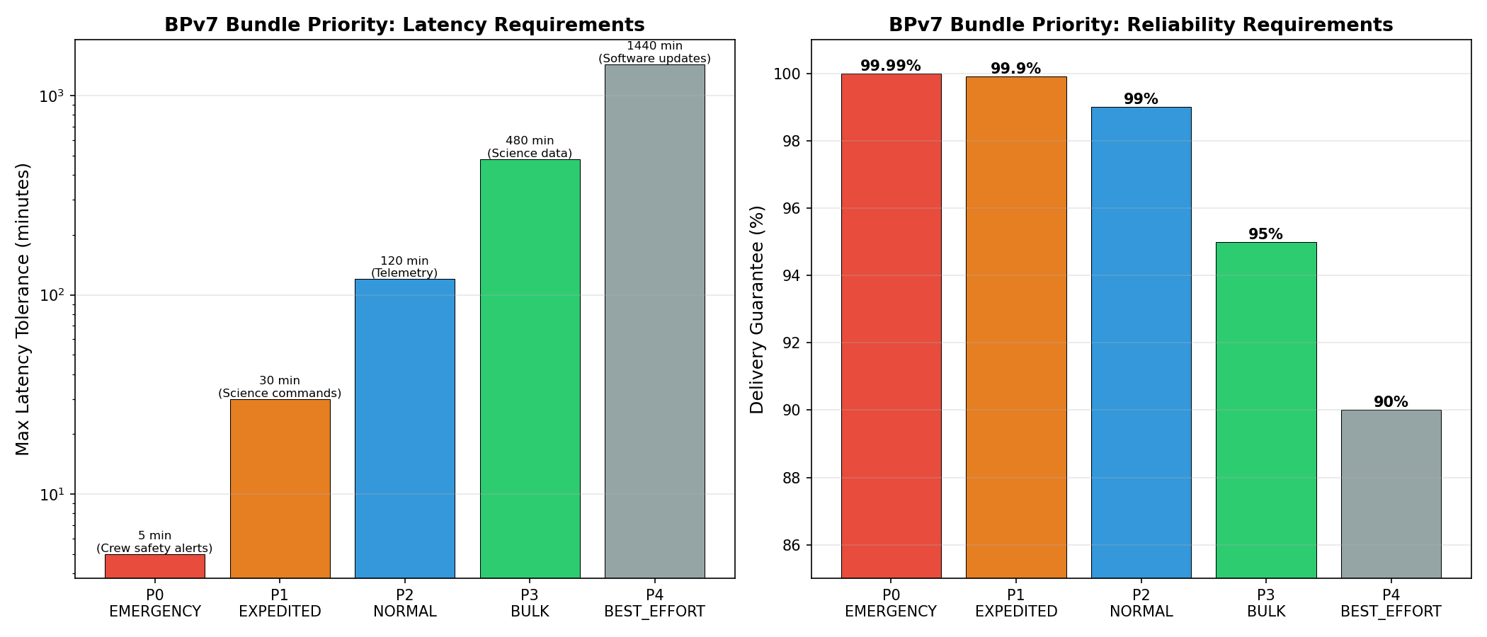
Breaks down bundle traffic by priority class (Emergency, High, Normal, Low, Bulk), showing how the DTN system triages time-critical vs. bulk data.
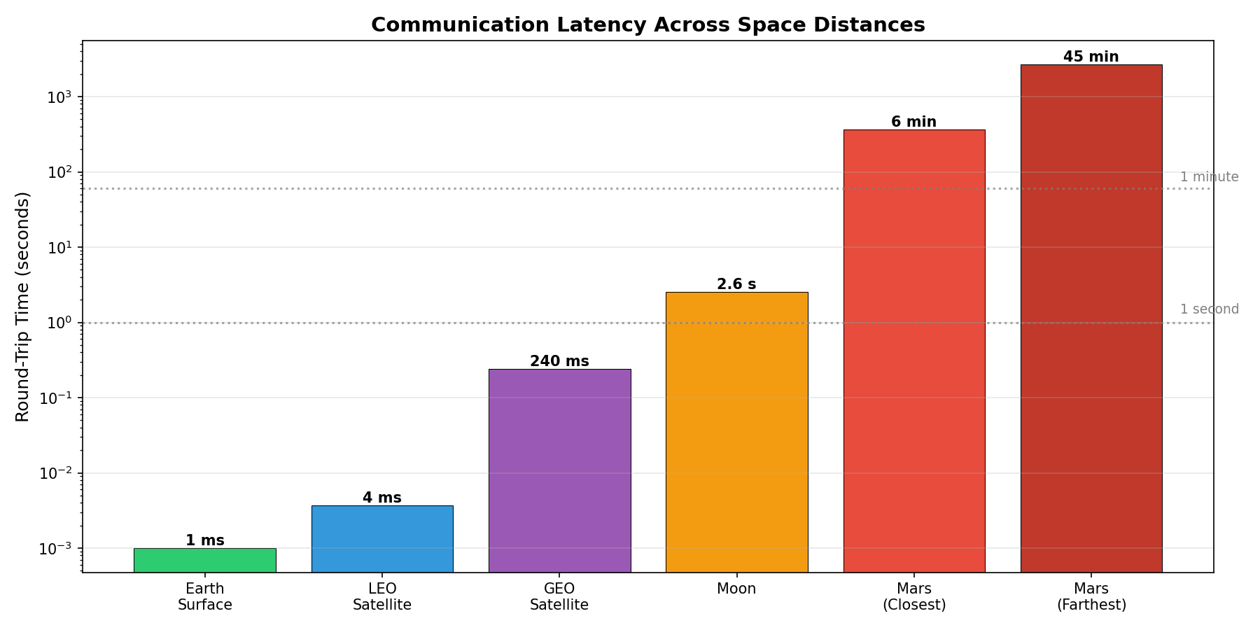
Bar chart comparing end-to-end bundle delivery latency across three routing approaches: static Contact Graph Routing, AETHERIX RL routing, and opportunistic flooding.
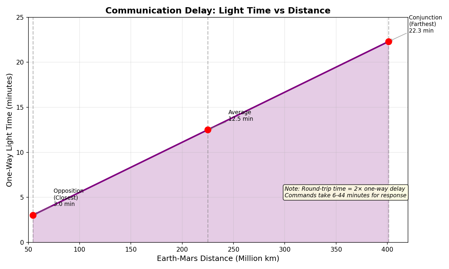
Maps one-way light-time delay from 3 minutes at opposition to 22 minutes at conjunction, the fundamental physics constraint on real-time communication.
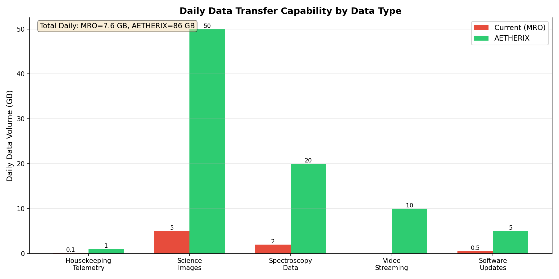
Projects cumulative data volume delivered over a 780-day mission, comparing AETHERIX throughput against current Mars relay capabilities.
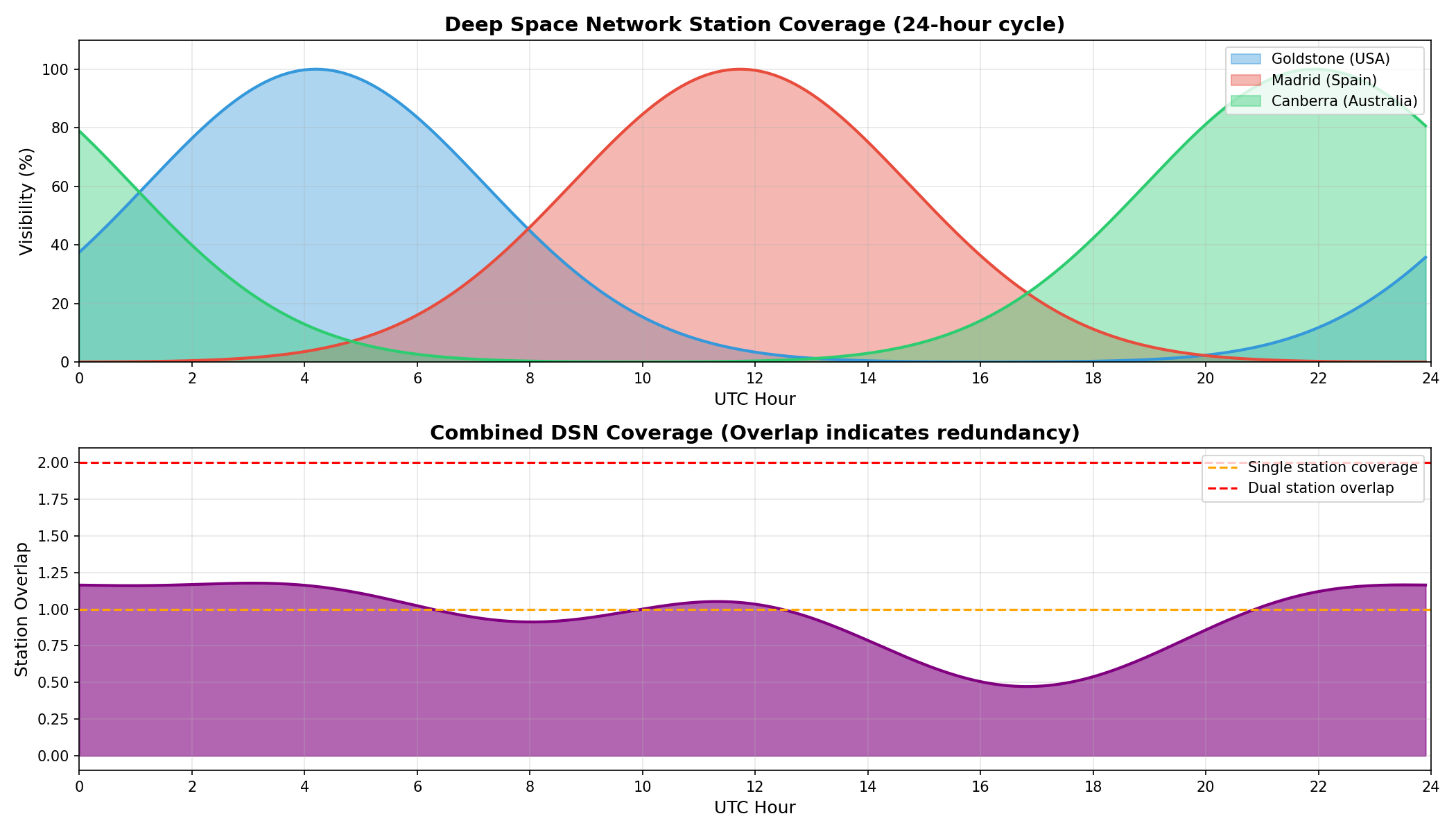
Visualizes Deep Space Network station visibility over 24 hours, showing how Goldstone, Madrid, and Canberra provide overlapping coverage.
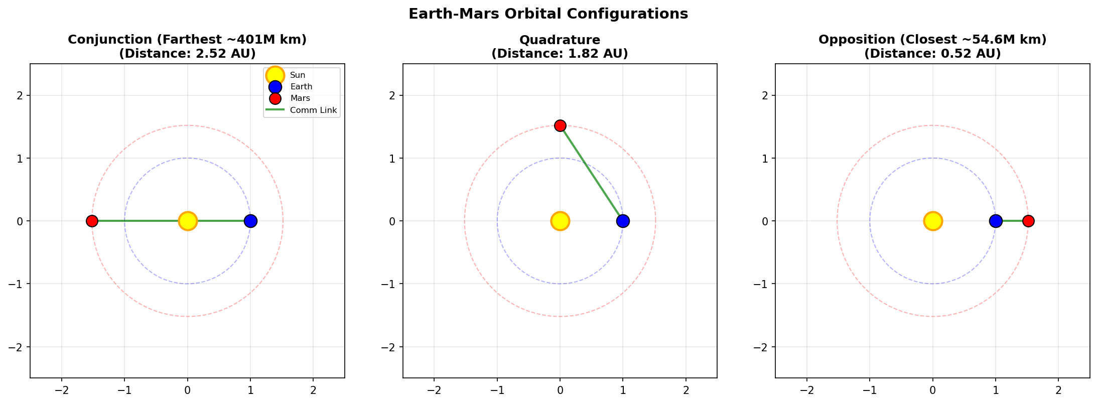
Two side-by-side orbital diagrams showing Earth and Mars at opposition (closest, 54.6 M km) and conjunction (farthest, 401 M km) relative to the Sun.
High-level system architecture showing all five AETHERIX modules — Infrastructure, Routing, Security, Orbital, and Simulation — with their CCSDS/RFC standards and inter-module data flows.
The complete five-tier network topology spanning Earth ground stations, Earth orbital relays, deep-space Lagrange-point relays, Mars orbital assets, and Mars surface nodes.
Step-by-step diagram of the DTN store-and-forward process: bundle creation, custody transfer, hop-by-hop forwarding with LTP reliability, and final delivery.
Illustrates the Earth-Mars communication path through all five network tiers, with distance markers and light-time delays at each hop.
End-to-end data flow from Mars surface sensor through the relay chain to Earth mission control, showing protocol processing at each node.
Layered protocol stack aligned against the CCSDS and IETF standards (BPv7, LTP, TCPCL/UDPCL), showing which protocol handles which communication segment.
Detailed node-level network topology with all 241 nodes and their inter-tier links, showing the full mesh of the AETHERIX backbone.
visualizations/scripts/. Download the full pack above for high-resolution versions suitable for presentations or reports.References & Standards
Every claim in this project traces to a cited standard, NASA mission dataset, peer-reviewed protocol, or verifiable source module.
Industry & Scientific [1]–[20]
Project Source [A1]–[A8]
python run_simulation.py
Al Nafi EduQual Level 6 oral examination — 3 Sep 2026, 84-minute session (presentation, live demo, examiner Q&A). Result published 8 Sep 2026. Full session record on NAFA-BOX → · ▶ Watch the recorded session & result details
Assessment Result
Al Nafi EduQual Level 6 oral examination — Diploma in Artificial Intelligence Operations, defending the AETHERIX project (Topic 59: Building Interplanetary Communication Network with Delay-Tolerant Networking, Quantum Communication, and Space-Based Infrastructure for Mars Mission Support). This page reports the verified outcome and the recorded session.
| Outcome | PASSED |
| Overall | 40.25 / 50 (80.5%) |
| Presentation component | 23 / 25 (92%) |
| Interview / Q&A component | 17.25 / 25 (69%) |
| Session | Oral examination · 1h 24m (presentation, live demo, examiner Q&A) |
| Assessed | 3 September 2026 |
| Result published | 8 September 2026 |
The companion study site (NAFA-BOX) rounds the overall result to 81%; the exact figure is 80.5% (40.25/50).
The full 84-minute assessment session as examined — presentation, live demo, and examiner Q&A. Also available on NAFA-BOX or YouTube.